Lecture 17: Forces and Energy Cost in Locomotion (Part 2)

Slide 1

• Continues directly from Lecture 16. Same overall theme — forces and mechanical energy demands of locomotion — now extending into the metabolic energy cost that follows from those force demands.

---

Slide 2

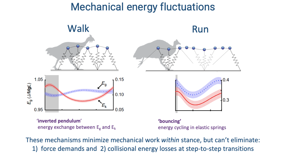
Recap — Mechanical Energy Patterns of Walking and Running

• Walking = inverted pendulum: stiff leg vaults the body up and over, exchanging gravitational potential (E_g) and kinetic energy (E_k) out of phase.
• Running = bouncing spring: compliant leg cycles mechanical energy through elastic springs in tendons and ligaments; E_g and E_k fluctuate in phase.
• These passive mechanisms minimize the muscular work within a stance, but they cannot eliminate:
  1. Force demands to support body weight against gravity.
  2. Collisional energy losses at step-to-step transitions.
• These two irreducible demands are what drive the metabolic energy cost of legged locomotion.

---

Slide 3

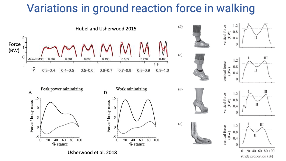
Walking GRF — Shape Variations with Speed, Strategy, and Footwear

• Speed dependence (Hubel & Usherwood 2015): the M-shape vertical GRF of walking deepens as speed rises. At very high walking speeds, the mid-stance trough can reach zero — and the body would be in aerial phase if walking continued, which is why a real walker switches gait first.
• Asymmetric M-shape (Usherwood et al. 2018): at high walking speeds the M-shape can become asymmetric. The shape depends on whether the gait is minimizing peak power (second peak smaller — prolongs the late-stance push-off so muscle-tendon units deliver power over longer time) or minimizing work (symmetric M — maintains passive inverted-pendulum motion).
• Foot morphology and footwear: the trace shape changes with how the foot meets the ground.
  • Plantigrade barefoot heel strike (typical human walking): an early impact peak appears, caused by the rapid heel-deceleration collision.
  • Forefoot or ball-of-foot contact (e.g., a human walking on the balls of the feet, or an ostrich digitigrade foot): the impact peak is smoothed out — collisional energy is absorbed by the longitudinal arch and elastic structures.
  • High-heel shoes: a stiletto removes the natural foot-roll, producing two sharp collisions (heel then toe) with no rolling in between, raising collisional cost. Platform heels are less disruptive than stilettos.

---

Slide 4

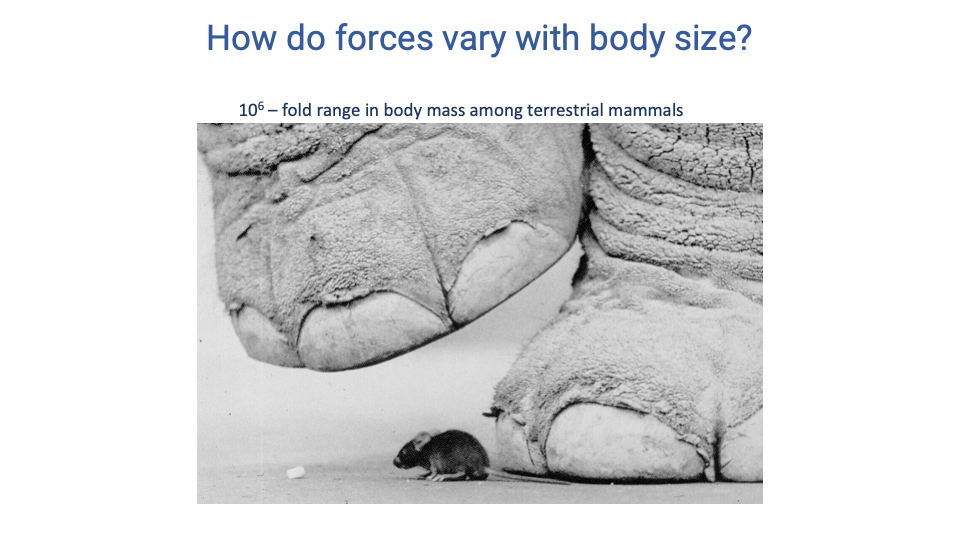
Body Size — A 10⁶-Fold Range Across Mammals

• Terrestrial mammals span ~10⁶-fold in body mass — from a few grams to several thousand kilograms.
• Different sizes pose different mechanical problems, and animals across this range show systematic differences in posture, limb proportions, and metabolic cost. These trends are explained by simple scaling arguments developed in the next slides.

---

Slide 5

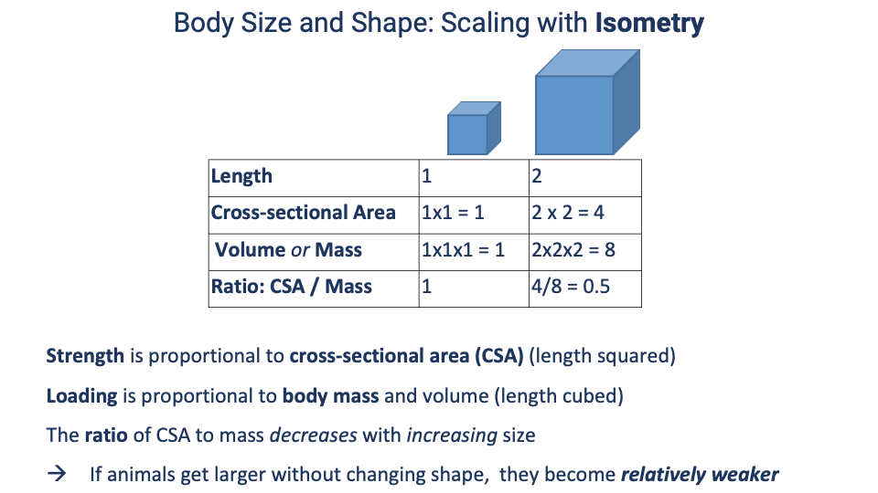
Isometric Scaling — Why Bigger Means Relatively Weaker

• Isometric scaling — if a body doubles in linear dimension (L) without changing shape:
  • Cross-sectional area (CSA) ∝ L² → strength of bones and muscles increases by 4×.
  • Volume and mass ∝ L³ → loading increases by 8×.
  • Ratio CSA/mass halves.
• Conclusion: strength scales with L², loading scales with L³ — so if animals enlarged without changing shape, larger animals would be relatively weaker.
• Real animals do not scale isometrically — they change shape with size (next slides). An elephant the size of a mouse with the same posture and bone proportions would simply be unable to support itself.

---

Slide 6

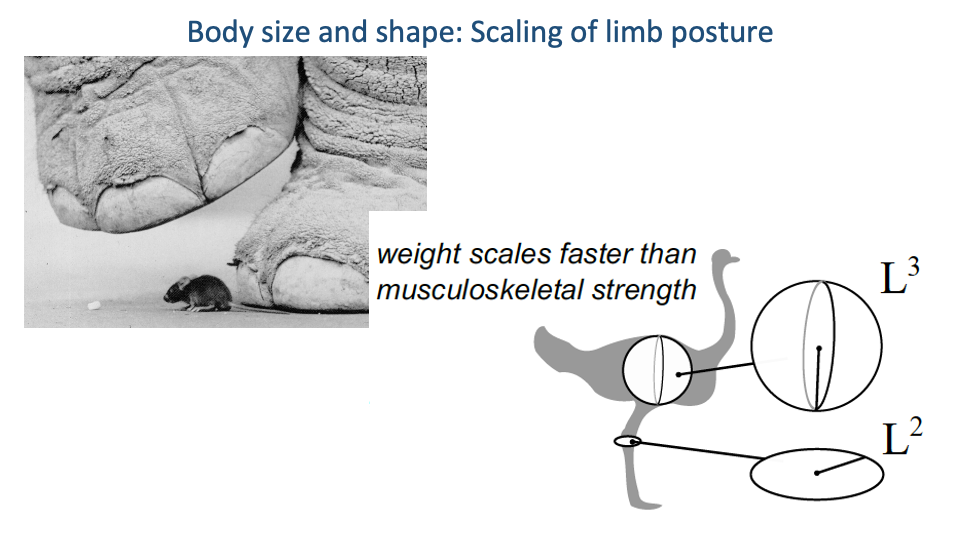
Posture Must Change with Size

• Because weight scales faster than musculoskeletal strength, larger animals cannot use the same posture as small animals.
• Solution: as body size increases, limb posture shifts to a more upright (extended) configuration, aligning the limb more closely with the ground reaction force.
• This raises the effective mechanical advantage (EMA) of the limb so that a given muscle force can resist a much larger GRF.

---

Slide 7

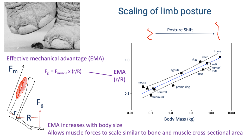
Effective Mechanical Advantage Scales with Body Size

• The EMA, defined as $r/R$ — the ratio of muscle moment arm $r$ to GRF moment arm $R$ — increases systematically with body mass across mammals.
• Quantitative result (Biewener and colleagues): EMA rises from ~0.1 in small rodents to ~1.0 in horses on a log-log line spanning four orders of magnitude in body mass.
• Mechanism — posture shift: large animals stand with a more upright (extended) limb; small animals with a crouched limb. The upright posture aligns the limb with the GRF, raising EMA.
• Functional consequence: with higher EMA, a given muscle force can resist a larger GRF. This allows muscle force capacity to keep up with body weight as size increases — so muscle and bone do not have to scale impossibly fast with body mass.
• Trade-off (revisited in the human-context lecture): a crouched posture, while metabolically expensive, gives greater range of joint motion and is therefore better for acceleration and maneuvering — which is why small animals run with crouched legs even though it is energetically costly.

---

Slide 8

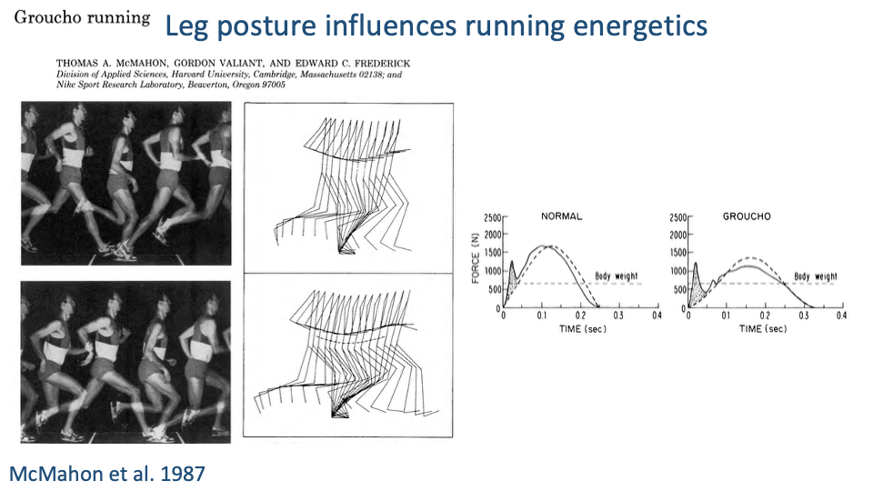
Groucho Running — Manipulating Posture in Humans

• Classic experiment (McMahon, Valiant & Frederick 1987): humans were asked to run with an artificially flexed (crouched) knee posture — the “Groucho” run — and compared with their normal running.
• GRF effects of crouched posture:
  • Longer contact time (broader force trace).
  • Lower peak vertical force but larger fore-aft (horizontal) excursions.
  • Greater joint flexion-extension range and more mechanical work at the joints.

---

Slide 9

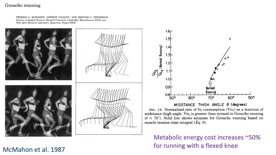
Crouched Running Costs ~50% More Metabolic Energy

• Same experiment, metabolic side: normalized VO₂ rose with the degree of knee flexion at mid-stance.
• At the most flexed postures, metabolic cost increased by ~50% above normal running.
• Demonstrates a tight link from posture → muscle force demand → metabolic cost: even small changes in geometry produce large changes in energy cost.
• Begs the question of why small animals voluntarily use crouched postures if they could save so much energy by extending their legs — addressed in the lecture by the trade-off between economy and maneuverability/acceleration.

---

Slide 10

Why GRF Matters

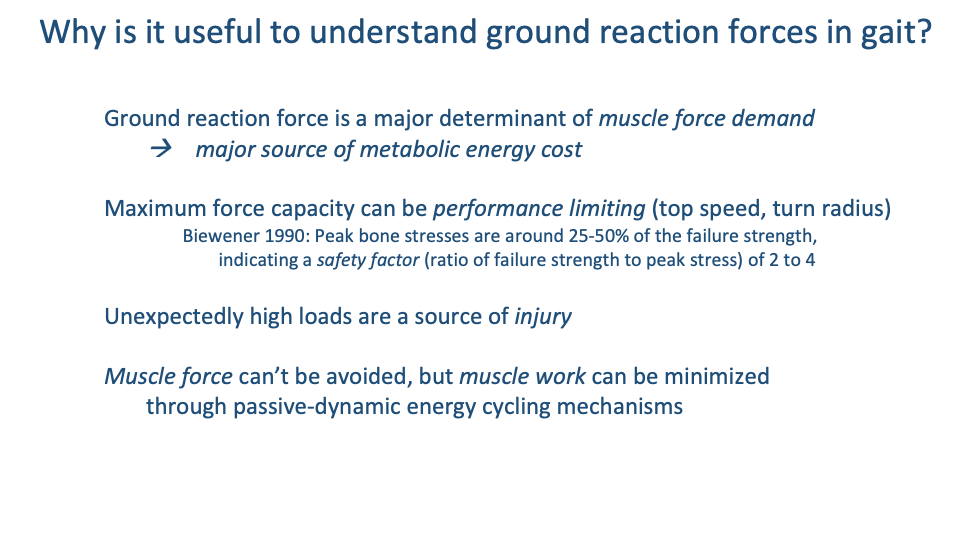
• Four reasons to care about ground reaction forces in gait:
  1. GRF is a major determinant of muscle force demand, and therefore a major source of metabolic energy cost.
  2. Maximum force capacity is performance limiting. Leg-extensor strength predicts top running speed in elite athletes and turn radius in rapid maneuvering.
  3. Bone safety factor (Biewener 1990): peak bone stresses in everyday locomotion are 25–50% of failure strength, giving a safety factor of 2–4 that is remarkably constant across vertebrates because bone remodels to match typical loads.
  4. Unexpectedly high loads cause injury. Knowing the typical loading helps explain which activities are most injury-prone.
• Force cannot be avoided (gravity is non-negotiable); muscle work can be minimized through inverted-pendulum and elastic-spring mechanisms (Slide 2).

---

Slide 11

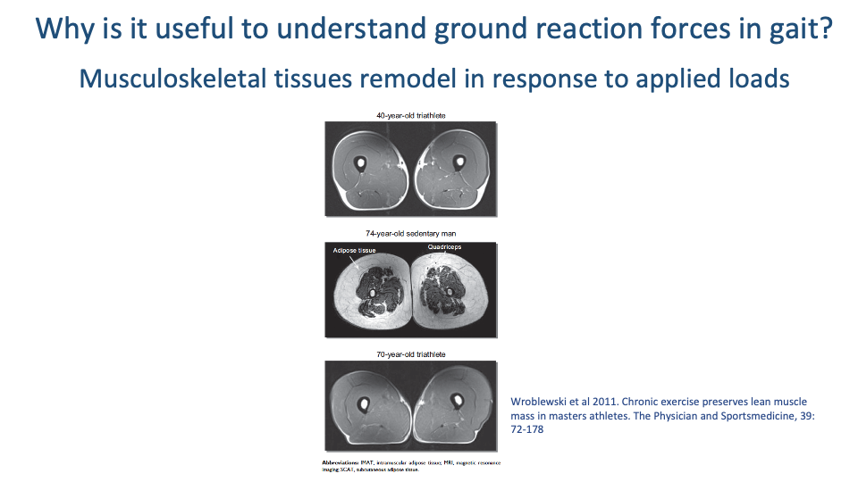
Tissues Remodel with Applied Load

• Cross-sectional MRI from Wroblewski et al. 2011 of three thighs: a 40-year-old triathlete, a 74-year-old sedentary man, and a 70-year-old triathlete.
• The 70-year-old triathlete has muscle and bone architecture nearly indistinguishable from the 40-year-old triathlete — and dramatically different from the 74-year-old sedentary subject.
• The biggest difference is not age but activity level. Chronic exercise preserves muscle mass and bone density by maintaining the mechanical loads that drive tissue remodeling.
• A practical motivation for the rest of the lecture: understanding the forces and energy costs of exercise lets us predict how training and lifestyle shape tissue health over the lifespan.

---

Slide 12

Learning Objectives

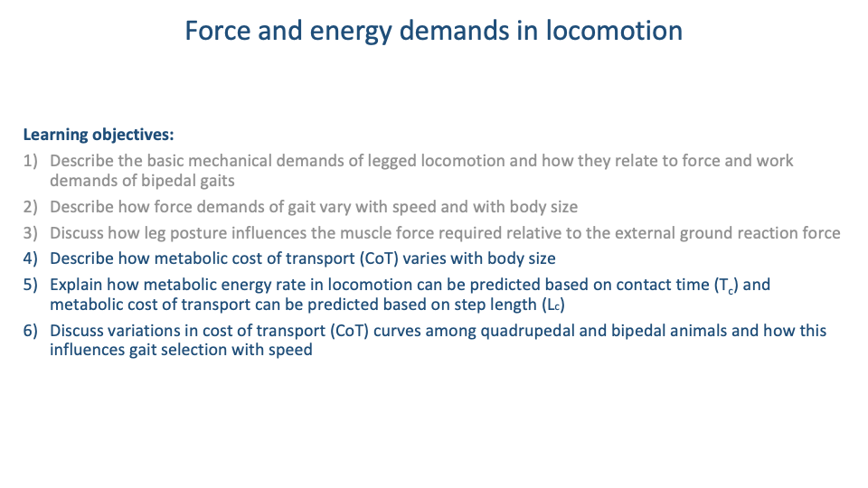
• The lecture covers six related objectives — the first three were largely set up in Lecture 16, and the last three are the focus of Lecture 17:
  1. Mechanical demands → force/work demands of bipedal gaits.
  2. Force demands vary with speed and body size.
  3. Leg posture sets the muscle force required for a given GRF.
  4. Cost of transport (CoT) varies with body size.
  5. Metabolic rate predicted from contact time (T_c); CoT predicted from step length (L_c).
  6. CoT curves vs. speed in quadrupeds and bipeds, and how those curves drive gait selection.

---

Slide 13

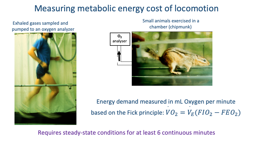
Measuring Metabolic Cost — Respirometry and the Fick Principle

• Energy cost of locomotion is measured indirectly as oxygen consumption ($\dot{V}O_2$), related to the Fick principle:

\[\dot{V}O_2 = \dot{V}_E (F_I O_2 - F_E O_2)\]

where $\dot{V}_E$ is the rate of expired air, and $F_I O_2$ and $F_E O_2$ are the inspired and expired oxygen fractions.

• Human set-ups use a face mask (or hood) sampling exhaled gases into an oxygen analyzer; small-animal set-ups seal the animal inside a chamber with a continuous airflow and sampled output.
• Key methodological constraint: respirometry requires steady-state conditions for at least ~6 minutes. This rules out instantaneous measurements during rapid maneuvers and limits classical CoT data to steady-state treadmill or overground locomotion.

---

Slide 14

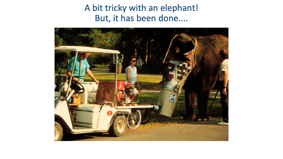
Respirometry — Even on an Elephant

• Brief and humorous: respirometry has been done on elephants by mounting a custom mask, putting the analysis equipment on a golf cart, and walking the cart-elephant pair around the zoo.
• Demonstrates that respirometry is in principle applicable across the full vertebrate body-size range — though logistically far easier in some species than others.

---

Slide 15

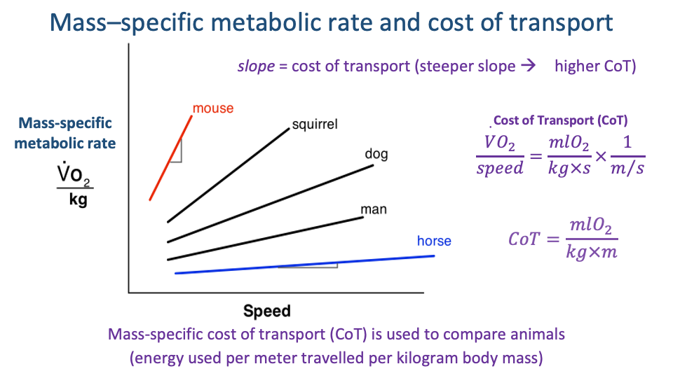
Mass-Specific Metabolic Rate and CoT

• Mass-specific metabolic rate $\dot{V}O_2/kg$ increases approximately linearly with speed within a gait.
• The slope of that line is the cost of transport:

\[\text{CoT} = \frac{\dot{V}O_2}{\text{speed}} = \frac{\text{ml }O_2}{\text{kg} \cdot \text{s}} \times \frac{1}{\text{m/s}} = \frac{\text{ml }O_2}{\text{kg} \cdot \text{m}}\]

• CoT is energy used per meter travelled per kg of body mass — the standard metric for comparing locomotor economy across species of very different size.
• Across mammals, the slope is steeper in small animals (mouse) and shallower in large animals (horse) — small animals are metabolically expensive per unit distance.

---

Slide 16

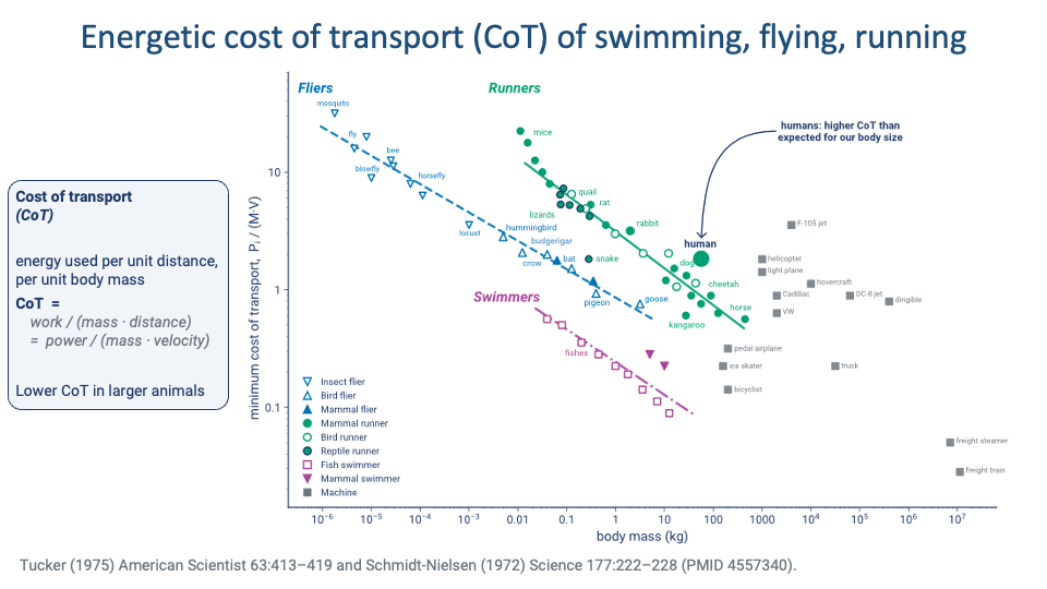
Cost of Transport Across Locomotor Modes

• The Tucker–Schmidt-Nielsen compilation places fliers, runners, and swimmers on a single log–log CoT vs. body-mass plot.
• Three universal patterns:
  • Swimmers are cheapest per unit distance — water supports body weight, eliminating the cost of weight-support.
  • Fliers are next — flapping is expensive but they cover distance fast.
  • Runners are most expensive per unit distance — full support against gravity plus collisional losses.
• Within each mode, larger animals have lower CoT.
• Humans sit above the runner trend line — our running is expensive for our body size (revisited in Lecture 18). We are not metabolically specialized runners — but our large body size still places us at a relatively low absolute CoT.
• Engineered machines (cars, trains, jets, hovercraft, helicopters) plotted in grey for comparison — most have higher CoT than animals in their size range.

---

Slide 17

Kram & Taylor 1990 — Cost Predicted by 1/T_c

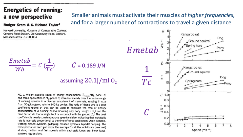
• Insight (Kram & Taylor 1990): across diverse species and speeds, mass-specific metabolic rate per body weight is predicted by a strikingly simple equation:

\[\frac{\dot{E}_{\text{metab}}}{W_b} = C \cdot \frac{1}{T_c}\]

where $T_c$ is the stance contact time of one foot per stride, and $C$ is a near-constant cost coefficient.

• C ≈ 0.189 J per N of body weight supported (assuming 20.1 J per mL O₂).
• Interpretation: the cost of generating force per Newton of support is relatively constant across species, but smaller animals must turn their muscles on and off at higher frequencies (shorter T_c) to keep up with the gait — and pay accordingly more energy per second.
• Bottom three panels (right): when plotted vs. speed, $\dot{E}_{\text{metab}}/W_b$ and $1/T_c$ both rise with speed and with decreasing body size, while C remains nearly constant — the equation captures most of the species-and-speed variation.

---

Slide 18

Oxycaloric Coefficients — Converting O₂ to Joules

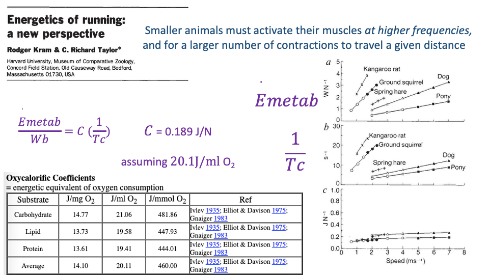
• Conversion factor used in the Kram-Taylor framework: ~20.1 J per mL O₂ — the average oxycaloric coefficient.
• The coefficient varies modestly with the substrate being oxidized:
  • Carbohydrate: ~21.1 J/mL O₂.
  • Lipid: ~19.6 J/mL O₂.
  • Protein: ~19.4 J/mL O₂.
  • Average: ~20.1 J/mL O₂.
• Differences are small because all aerobic pathways extract similar energy per oxygen atom consumed. 20.1 J/mL O₂ is the default conversion factor used throughout comparative energetics.

---

Slide 19

Larger Animals Travel Farther Per Stride

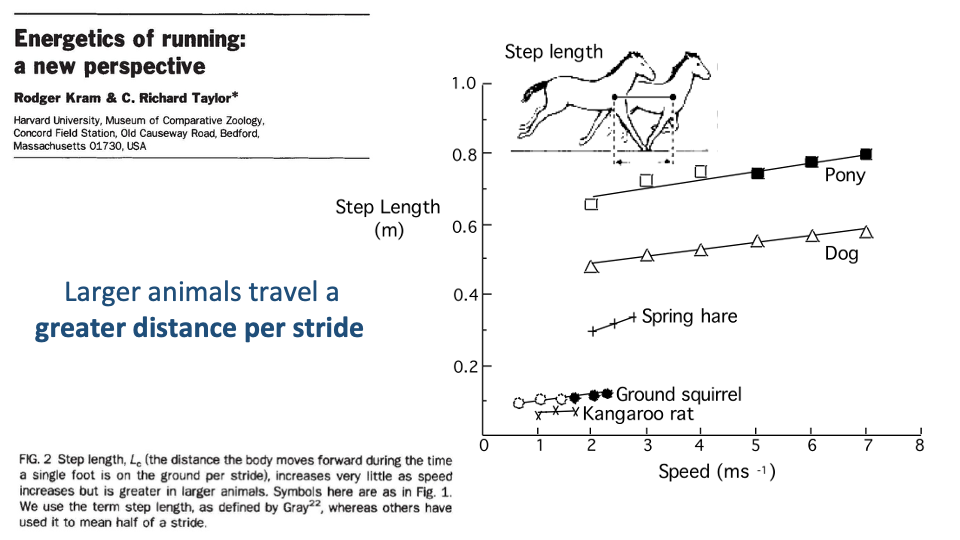
• Step length (L_c) — the distance the body moves forward during one stance — is proportional to body size.
• A pony covers ~0.8 m per step; a kangaroo rat about 0.1 m. Within any species, L_c rises modestly with speed; across species, the dominant predictor is body size.
• This is the second half of the Kram-Taylor explanation for the decrease in CoT with body size: large animals not only contract muscles less frequently, but each contraction also moves them farther.

---

Slide 20

CoT Predicted by 1/L_c

• Combining the previous two slides:

\[\frac{E_{\text{cot}}}{W_b} = C \cdot \frac{1}{L_c}\]

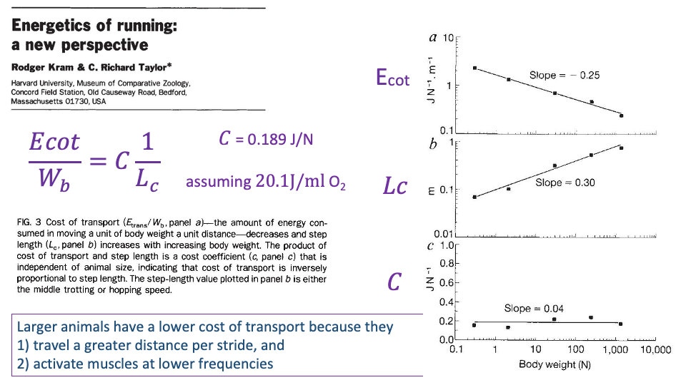
CoT per Newton of body weight equals the cost coefficient divided by step length.

• Scaling exponents:
  • CoT vs. body weight: slope ≈ −0.25 (CoT falls with size).
  • L_c vs. body weight: slope ≈ +0.30 (step length rises with size).
  • C vs. body weight: slope ≈ +0.04 (cost coefficient is essentially constant).
• Take-home (Kram & Taylor): larger animals have lower CoT for two compounding reasons:
  1. They travel farther per stride (larger L_c).
  2. They activate muscles at lower frequencies (longer T_c).
• The same logic applies within humans: individuals with longer legs tend to have lower CoT than shorter-legged individuals.

---

Slide 21

Transition — CoT vs. Speed Within Gait

• Section transition. The previous slides covered how CoT scales with body size at a preferred speed. The next set asks how CoT changes with speed within each gait, and how it sets the gait-transition speeds.

---

Slide 22

Horses — Energy Cost Across Walk, Trot, and Gallop

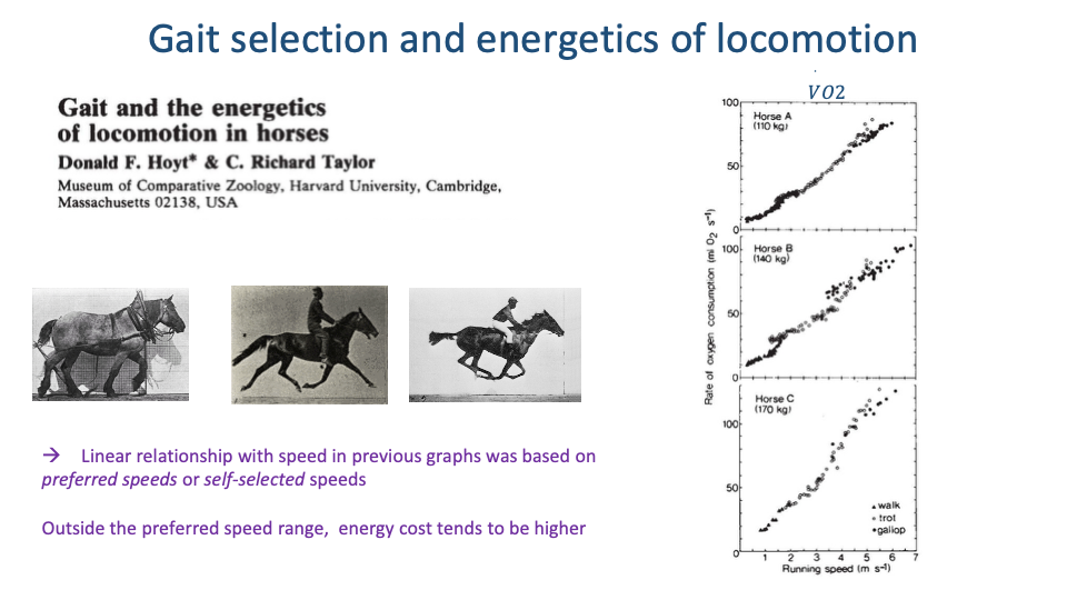
• Hoyt & Taylor 1981 trained horses to use walk, trot, and gallop over wide speed ranges, including speeds they would not naturally use for each gait.
• The classic linear $\dot{E}_{\text{metab}}$-vs-speed relationships of earlier studies were based on preferred (self-selected) speeds only — and so missed within-gait curvature.
• When horses were forced to use a gait at non-preferred speeds, $\dot{V}O_2$ rose non-linearly: energy cost was higher outside the preferred speed range of each gait.

---

Slide 23

CoT Within Each Gait — U-Shaped Curves

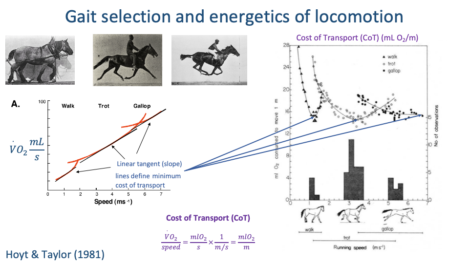
• For each gait, CoT vs. speed forms a U-shaped curve with a clear minimum.
• The slope of a line from the origin to a point on the $\dot{V}O_2$-vs-speed curve equals CoT at that speed. The line tangent from the origin marks the minimum-CoT speed for that gait.
• For horses, the minimum-CoT speed within each gait corresponds closely to the preferred (voluntarily chosen) speed — confirmed by overground speed histograms aligning with the U-curve minima.

---

Slide 24

Two Rules of Gait Selection

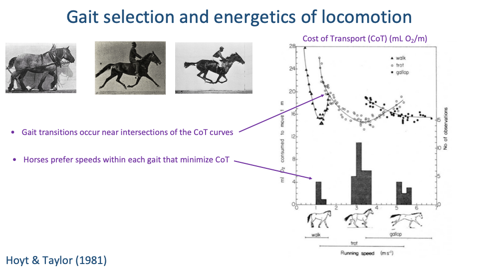
• Two simple rules emerge from the Hoyt-Taylor curves:
  1. Gait transitions occur near the intersections of the CoT curves — the speed at which one gait becomes more expensive than the next.
  2. Animals choose speeds within each gait that minimize CoT — preferred speed sits near the U-curve minimum.
• Energetics is a strong (though not the only) driver of voluntary gait and speed selection in steady locomotion.

---

Slide 25

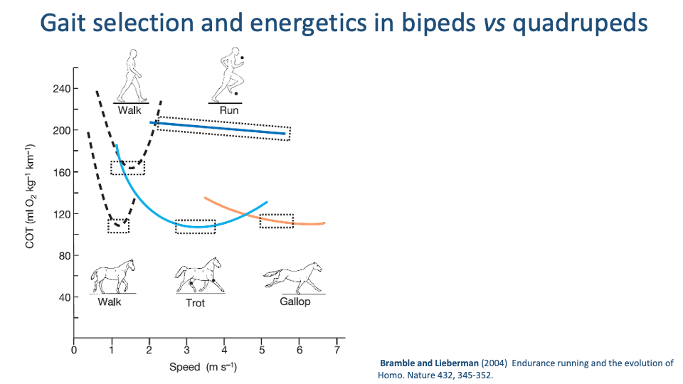
Bipeds vs. Quadrupeds — Walking U, Running Flat

• A composite CoT-vs-speed plot from Bramble & Lieberman 2004 places humans and horses on the same axes.
• Walking (in both humans and horses): a steep U-shaped curve with a clear minimum.
• Running in humans: nearly flat — CoT changes very little with running speed, an unusual feature relative to quadrupeds.
• Quadrupeds show three overlapping U-shaped curves (walk, trot, gallop), with gait transitions at the curve intersections — exactly the Hoyt-Taylor pattern.
• Human running has no comparable equivalent. We commit to a single bouncing gait (running) and can use a wide speed range without paying much extra energy.

---

Slide 26

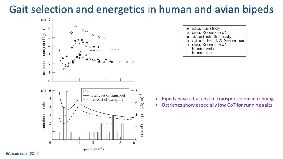
Avian Bipeds — Flat Running CoT, Ostriches Especially Cheap

• Watson et al. 2011 measured net CoT for emus, ostriches, and rheas over a wide speed range, alongside human walk and run reference curves.
• All bipeds — human and avian — show flat running CoT at running speeds. The plateau is a general feature of bipedal running, not just a human quirk.
• Ostriches sit at especially low running CoT (~1.5–2 J kg⁻¹ m⁻¹) — they are exceptional running specialists.
• Voluntary overground speeds (bottom panel) cluster near the minimum of the CoT curve — the same Hoyt-Taylor pattern, now in birds.

---

Slide 27

Reduced-Gravity Experiments — Method

• Farley & McMahon 1992: human subjects ran on a treadmill while a ceiling-mounted spring system applied a constant upward force, effectively lowering apparent gravity (and therefore body weight).
• Manipulating gravity isolates the weight-support cost from other components of locomotion: at the same speed, a runner at 0.5g supports half as much weight against gravity.
• The right-hand plots show:
  • Mass-specific metabolic rate (Panel A) is much lower at 0.5g than at 1g across all speeds.
  • CoT (Panel B) is roughly halved at 0.5g.
• A direct experimental confirmation of the Kram-Taylor framework: when body weight is reduced, force demand drops, and metabolic cost falls in proportion.

---

Slide 28

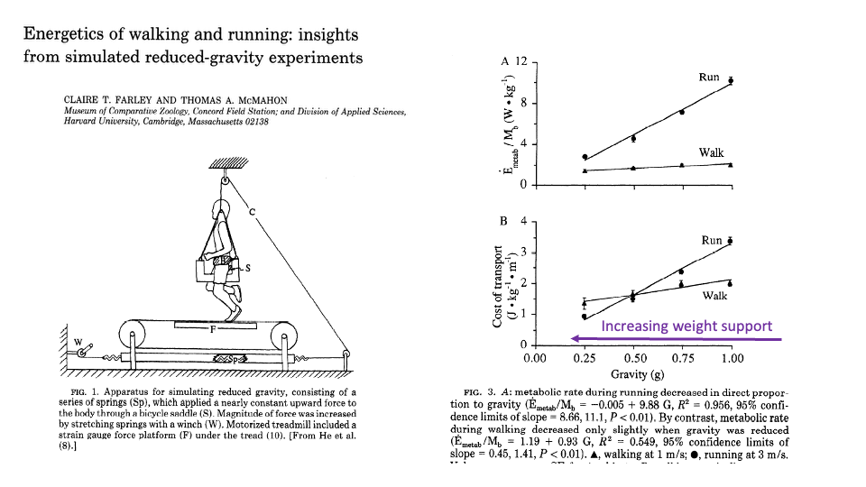
Reduced-Gravity — Walking vs. Running Have Different Sensitivities

• Plotting metabolic rate and CoT against gravity (g) at fixed speed reveals a striking dissociation:
  • Running cost falls in near-direct proportion to gravity (slope ≈ 9.9 W kg⁻¹ per g, R² = 0.96). Reducing weight support by half cuts running cost nearly in half.
  • Walking cost falls only modestly with reduced gravity (slope ≈ 0.93 W kg⁻¹ per g, R² = 0.55).
• Mechanistic interpretation:
  • Running cost is dominated by the force demand to support body weight at each landing — reducing weight directly reduces force.
  • Walking cost is dominated by mechanical work to redirect the center of mass (collisional losses at step-to-step transitions) — this work depends weakly on weight support.
• Powerful confirmation that running and walking are limited by different physical demands, and that the Kram-Taylor force-cost framework applies specifically to running and other bouncing gaits.

---

Slide 29

Limitations of Classic Steady-State Locomotion Studies

• The classic respirometry framework requires steady-state locomotion for at least ~6 minutes — so all of the data on Slides 13–28 are from constant-speed treadmill or controlled overground trials.
• Two important limits:
  • Real-world locomotion is rarely steady-state. Foraging, commuting, sport, and everyday walking involve frequent starts, stops, turns, and terrain changes that the steady-state framework cannot directly assess.
  • Sample sizes are small and rarely capture individual variation in size, leg length, fitness, age, or terrain experience.
• Modern wearables and IMU/respirometry systems make it possible to address both limits (next slides).

---

Slide 30

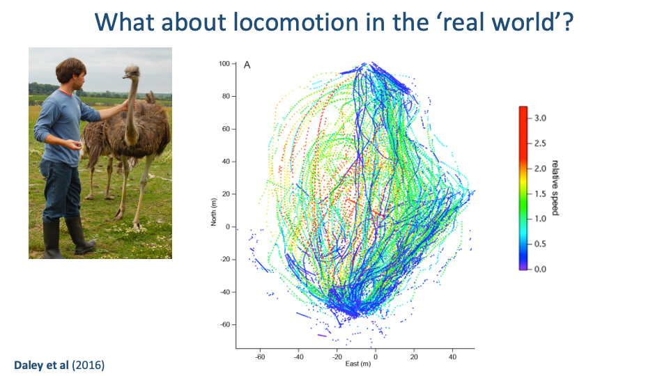
Tracking Real-World Movement — Ostriches

• Daley et al. 2016 instrumented free-ranging ostriches with IMU and GPS sensors to track foot trajectories and speeds across a large outdoor enclosure.
• The trajectory map shows that real movement is highly variable in speed, direction, and turning — nothing like the constant-treadmill paradigm.
• Real locomotor energetics may differ substantially from steady-state lab estimates, especially in habitats with frequent turns, terrain variation, or social interactions.

---

Slide 31

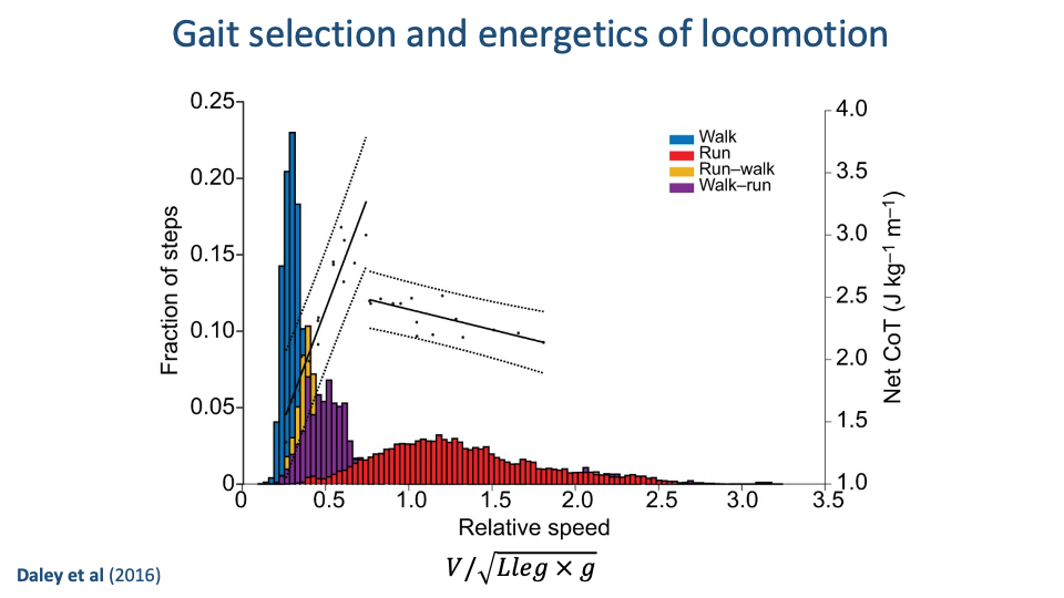
Real-World Speed Distributions and CoT

• For free-ranging ostriches, the distribution of step relative speeds (V / √(L_leg · g)) shows that:
  • Most steps fall in the slow walking range (relative speed ~0.3) — corresponding to the minimum-CoT walking speed.
  • There is a broad running distribution centered at higher relative speeds — corresponding to the flat-CoT running plateau.
  • Transitional gaits (run-walk, walk-run) are rare and brief.
• The CoT data overlaid on the histogram confirm that ostriches voluntarily choose the relative speeds that minimize CoT within each gait — Hoyt-Taylor extended to free-ranging birds.

---

Slide 32

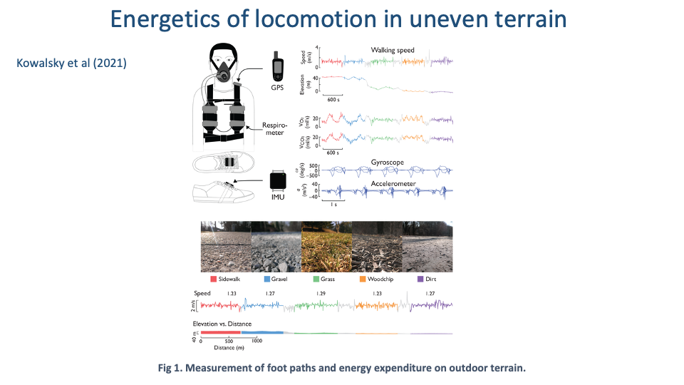
Wearable Tools for Real-World Energetics

• Kowalsky et al. 2021 used a portable respirometer + GPS + IMU setup to measure energy expenditure during walking across five real terrains: sidewalk, dirt, gravel, grass, woodchips.
• This is the modern answer to the classical lab limitation: wearable instrumentation lets researchers measure CoT and gait variability in the field, across varying terrain, and in larger and more diverse subject populations.

---

Slide 33

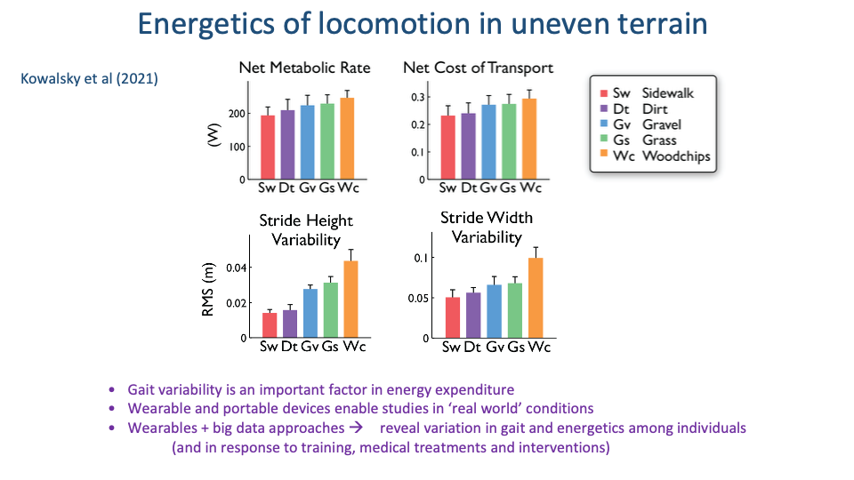
Uneven Terrain Raises CoT in Proportion to Gait Variability

• Across the five terrains, both stride-height variability and stride-width variability increase going from sidewalk to woodchips.
• Net CoT increases in parallel, by ~25% from sidewalk to woodchips.
• Two implications:
  • Gait variability is itself a metabolic cost. Stabilizing each step on uneven ground demands additional muscle activation that adds to the steady-state baseline.
  • Wearable + big-data approaches enable comparisons across individuals (training status, age, medical condition, intervention) — extending the comparative-energetics framework from species to individuals.

---

Slide 34

Learning Objectives Revisited

• Closing repeat of the learning objectives. Each is now backed by data from the lecture:
  1. Mechanical demands → force and work demands.
  2. Force varies with speed and body size.
  3. Posture sets the muscle force needed.
  4. CoT decreases with body size.
  5. Metabolic rate predicted by 1/T_c; CoT predicted by 1/L_c.
  6. CoT-vs-speed curves drive gait selection in quadrupeds and bipeds.

---

Slide 35

Summary

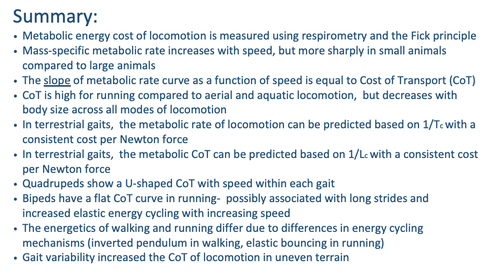
• Final summary of the lecture in ten bullets:
  • Respirometry and the Fick principle measure the metabolic energy cost.
  • Mass-specific metabolic rate increases with speed, more steeply in small animals.
  • The slope of metabolic rate vs. speed is the CoT.
  • Running is more expensive per distance than flying or swimming, but CoT decreases with body size in all three modes.
  • In terrestrial gaits, metabolic rate is predicted by 1/T_c and CoT by 1/L_c, with a near-constant cost per Newton of force.
  • Quadrupeds show U-shaped CoT curves within each gait.
  • Bipeds (humans and birds) have flat running CoT curves, possibly because long strides and elastic cycling rise together with speed.
  • Walking and running have different physics — inverted pendulum vs. elastic bouncing — and respond differently to weight support (reduced-gravity experiments).
  • Real-world gait variability raises CoT — captured by modern wearable studies of free locomotion.

---

Key Equations

Equation	Name	Description
$\dot{V}O_2 = \dot{V}_E (F_I O_2 - F_E O_2)$	Fick principle	Oxygen consumption equals ventilation rate times the difference between inspired and expired O2 fractions. The basis of respirometry.
$\text{CoT} = \dot{V}O_2 / \text{speed}$	Mass-specific cost of transport	Energy used per unit distance traveled, per unit body mass — typically expressed as mL O2 kg−1 m−1 or J kg−1 m−1.
$\dot{E}_{\text{metab}}/W_b = C \cdot (1/T_c)$	Kram & Taylor metabolic rate equation	Mass-specific metabolic rate per body weight equals the cost coefficient $C$ divided by stance contact time $T_c$. $C ≈ 0.189$ J/N is nearly constant across mammals.
$E_{\text{cot}}/W_b = C \cdot (1/L_c)$	Kram & Taylor cost-of-transport equation	CoT per unit body weight equals the cost coefficient $C$ divided by step length $L_c$. Larger animals have longer Lc, so lower CoT.
$F_g = F_{\text{muscle}} \cdot (r/R)$	Effective mechanical advantage	The ground reaction force a leg can resist equals the muscle force times the ratio of muscle moment arm to GRF moment arm. EMA increases with body size.
$1 \text{ mL } O_2 \approx 20.1 \text{ J}$	Oxycaloric coefficient	Average energetic equivalent of aerobic oxygen consumption. Converts respirometry data to joules of energy expenditure.

---

Glossary of Key Terms

Term	Definition
Cost of transport (CoT)	Energy used per unit distance traveled, per unit body mass. Standard metric for comparing locomotor economy across species and speeds. SI units: J kg−1 m−1.
Mass-specific metabolic rate	Rate of energy use per unit body mass during locomotion. The slope of metabolic rate vs. speed gives CoT. Increases more steeply with speed in small animals than in large animals.
Stance (contact) time, Tc	Duration that one foot is in contact with the ground during a single step. Small animals have short Tc and must therefore activate muscles at higher frequencies.
Step length, Lc	Distance the body moves forward during one stance. Increases with body size; longer Lc → lower CoT in the Kram & Taylor framework.
Cost coefficient (C)	Energy used per Newton of body weight supported, per second. ~0.189 J/N, approximately constant across species and speeds.
Oxycaloric coefficient	Energy released per unit oxygen consumed during aerobic metabolism. ~20.1 J/mL O2 on average (~21 J/mL O2 for carbohydrate, ~19.6 J/mL O2 for lipid). Used to convert respirometry data to joules.
Fick principle (respirometry)	The conservation principle linking ventilation, gas concentrations, and oxygen consumption — the foundation of indirect calorimetry.
Effective mechanical advantage (EMA)	Ratio of muscle moment arm to ground-reaction-force moment arm at a joint: EMA = r/R. Scales positively with body mass across mammals.
Plantigrade / digitigrade / unguligrade posture	Three foot postures along a continuum of distal-limb elongation. Plantigrade (humans, bears) — flat foot on ground; digitigrade (dogs, cats, birds) — toes on ground; unguligrade (horses, ungulates) — only the tips of the toes on ground. Larger and more cursorial animals are progressively more digitigrade or unguligrade.
Posture shift with body size	The trend across mammals for limb posture to become more upright with increasing body size, raising EMA so that muscle force can keep up with body weight.
Inverted-pendulum walking	Walking gait in which a relatively stiff leg vaults the body up and over with Eg and Ek exchanged out of phase, minimizing muscular work within stance.
Bouncing (elastic) running	Running gait in which a compliant leg cycles mechanical energy through elastic tendons and ligaments, with Eg and Ek in phase.
Collisional energy loss	The energy dissipated at the moment of foot-ground contact during step-to-step transitions. A major irreducible energy cost in legged locomotion; foot morphology and step length both modulate its size.
M-shaped vertical GRF	Characteristic double-hump vertical force trace of walking, with peaks at early and late stance and a mid-stance trough. Becomes asymmetric at high walking speed depending on whether peak power or peak work is minimized.
Groucho running	Voluntarily flexed-knee running posture used as an experimental probe. Raises GRF contact time, lowers peak vertical force, and increases metabolic cost by up to ~50%.
Bone safety factor	Ratio of bone failure strength to peak bone stress during typical locomotion. About 2–4 across vertebrates, because bone remodels to match the loads it routinely experiences.
Hoyt-Taylor rule	Across speeds within a gait, animals voluntarily choose the speed near the minimum of the U-shaped CoT curve, and switch gaits near CoT-curve intersections.
Flat running CoT	The pattern observed in bipeds (humans and birds) of CoT changing little with running speed over a wide range. Unlike quadrupeds, bipeds commit to one bouncing gait across most running speeds.
Reduced-gravity experiments	Treadmill experiments with a partial-weight suspension system that reduces apparent body weight. Demonstrate that running metabolic cost is approximately proportional to gravity, while walking cost is largely insensitive — confirming that running is force-limited and walking is work-limited.
Wearable respirometry and IMU	Portable equipment that allows measurement of $\dot{V}O_2$, GPS speed, and stride mechanics in real-world conditions. Enables comparisons across terrains and individuals beyond the steady-state lab paradigm.
Gait variability	Variation in stride length, step width, foot height, or timing from step to step. Increases on uneven terrain and raises CoT proportionally — an irreducible cost of stabilizing each step.