Week 7 Friday Review and Discussion
Slide 1

- Friday review and discussion session for Week 7: Training Effects on Muscle and Forces in Locomotion.
- Wraps up loose ends from Monday’s training lecture (evidence-quality questions, a case study on muscle cramps) and then provides an extended hands-on review of muscle work loops and muscle–tendon interactions through two recent research papers.
Slide 2
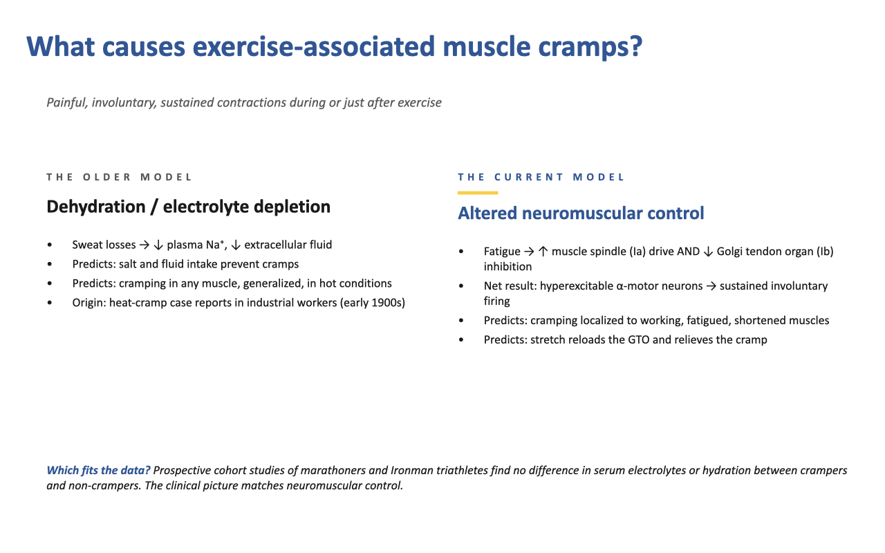
Two Competing Models of Exercise-Associated Muscle Cramps
- Working definition: painful, involuntary, sustained contractions during or just after exercise.
- Older model — dehydration / electrolyte depletion:
- Mechanism: sweat losses reduce plasma Na+ and extracellular fluid volume.
- Predictions: salt and fluid intake prevent cramps; cramping should be generalized across muscles and especially common in hot conditions.
- Origin: heat-cramp case reports in industrial workers in the early 1900s.
- Current model — altered neuromuscular control:
- Mechanism: muscle fatigue increases muscle-spindle (Ia) drive and decreases Golgi-tendon-organ (Ib) inhibition; the net effect is hyperexcitable α-motor neurons that fire involuntarily and sustainedly.
- Predictions: cramping is localized to muscles that are working, fatigued, and shortened; passive stretch reloads the GTO and relieves the cramp.
- Which model fits the data? Prospective cohort studies of marathoners and Ironman triathletes find no difference in serum electrolytes or hydration between crampers and non-crampers. The localization and stretch-relief patterns observed clinically also match the neuromuscular-control model.
Slide 3
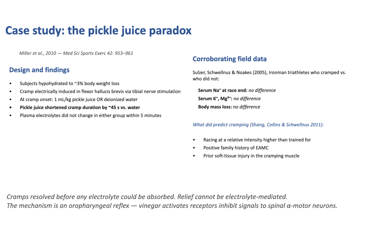
Case Study — The Pickle Juice Paradox
- Miller et al. 2010 design: hypohydrate subjects to ~3% body-weight loss, then electrically induce a cramp in the flexor hallucis brevis via tibial-nerve stimulation. At cramp onset, give either 1 mL/kg pickle juice or deionized water.
- Key finding: pickle juice shortened cramp duration by ~45 seconds vs. water — yet plasma electrolytes did not change in either group within the 5-minute observation window.
- Implication: the cramp resolved before any electrolyte could even be absorbed. The relief mechanism cannot be electrolyte-mediated. The current best explanation is an oropharyngeal reflex — vinegar activates receptors in the mouth and pharynx that send inhibitory signals to spinal α-motor neurons, breaking the involuntary firing pattern.
- Corroborating field data (Sulzer, Schwellnus & Noakes 2005): in Ironman triathletes, serum Na+, K+, Mg2+, and body-mass loss were not different between crampers and non-crampers at race end.
- What does predict cramping (Shang, Collins & Schwellnus 2011): racing at a relative intensity higher than trained for, a positive family history of exercise-associated muscle cramps, and a prior soft-tissue injury in the cramping muscle.
- The case study highlights two broader lessons:
- A famous folk remedy can give a real clue to a mechanism — but only after the data rule out the obvious explanation.
- Localized fatigue and motor-neuron control, not whole-body fluid/electrolyte status, are the dominant drivers of exercise-associated cramping.
Slide 4

Evaluating the Quality of Evidence
- Google Scholar indexes everything, including predatory journals and so-called gray literature. Indexing alone is not a quality filter.
- A working checklist for evaluating exercise-physiology evidence:
- Indexed in PubMed — at minimum, the journal has met PubMed’s editorial standards.
- Well-cited and not retracted — citations alone are not enough; retracted papers can continue to accumulate citations long after retraction.
- Sufficient and representative samples — small or non-representative samples (e.g., 20-year-old male athletes) cannot support general claims about all humans.
- No over-generalization from limited evidence — a single small study is rarely definitive.
- No obvious conflicts of interest — authors selling a related supplement or device are a red flag.
- Systematic reviews and meta-analyses are the gold standard — they use keyword searches, apply quality filters, and synthesize across many high-quality studies, giving more reliable conclusions than any single paper.
- Why this matters: a major learning objective of this course is to be able to answer questions yourself by probing the scientific literature, critically evaluate the evidence, and effectively synthesize what you find. This toolset is increasingly important in the modern publication era, where the rapid growth of gray-literature “noise” — predatory journals, preprints used out of context, supplement-marketing dressed as research — makes filtering for quality a core scientific skill rather than an optional one.
Slide 5
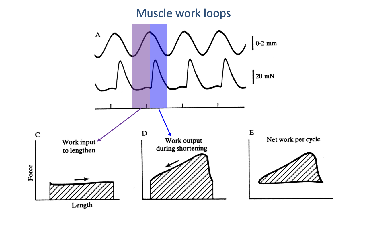
Building a Work Loop from Length and Force Traces
- A work loop is a plot of muscle force (y) vs. muscle length (x) over one complete contraction cycle. The plot encodes everything about the mechanical work the muscle does and the direction in which it flows.
- Construction (Panel A): the muscle is driven through a sinusoidal length cycle while a force trace is recorded.
- Purple-shaded band (stretch) — length is increasing. The area under the force-vs-length trace here is work input into the muscle (Panel C).
- Blue-shaded band (shortening) — length is decreasing. The area under the force-vs-length trace here is work output by the muscle (Panel D).
- The net work per cycle (Panel E) is the enclosed area of the closed loop — the difference between the shortening work and the lengthening work.
- Sign convention:
- Force higher during shortening than during lengthening → loop traced counterclockwise → net positive work (motor).
- Force higher during lengthening than during shortening → loop traced clockwise → net negative work (brake).
- Same force in both directions → enclosed area = 0 → muscle is acting as a strut/spring with no net mechanical work.
Slide 6
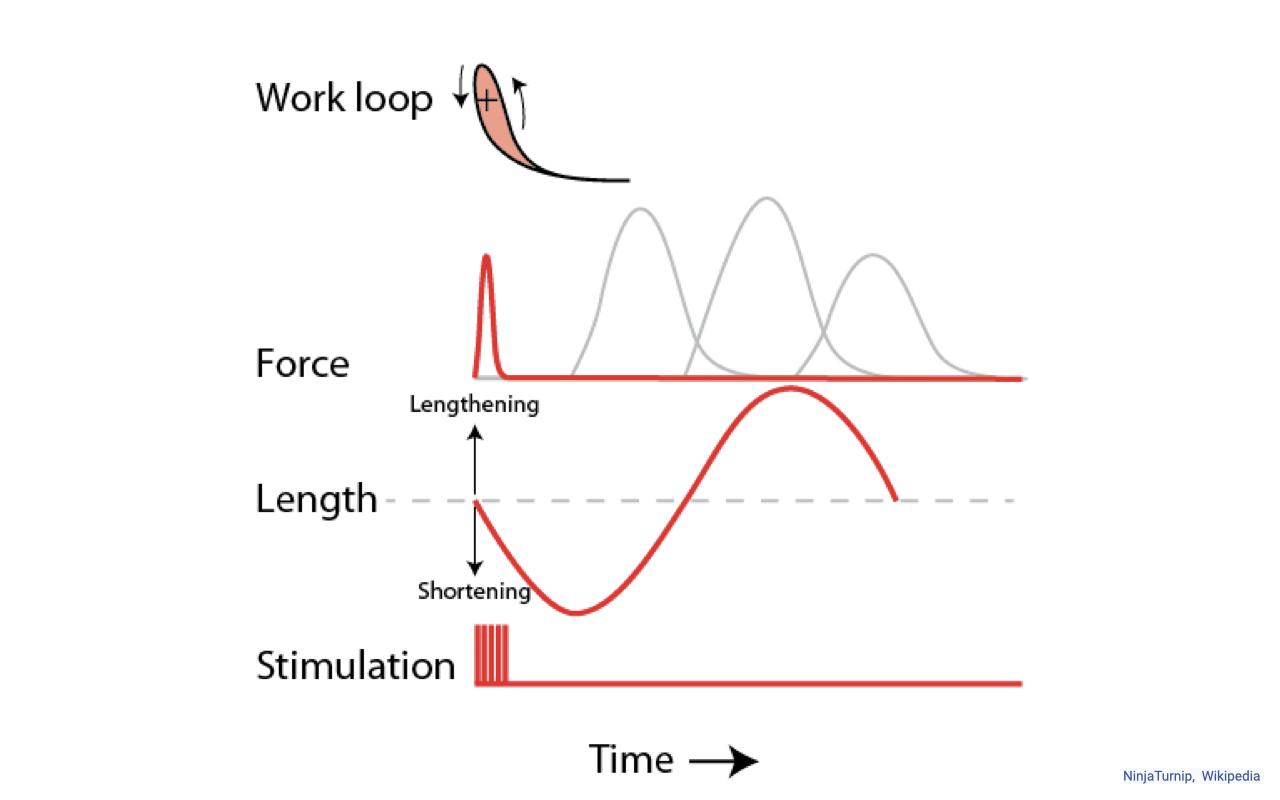
Stimulation Timing Shapes the Work Loop
- Same length trajectory, different stimulation timing → very different work-loop shapes and very different net work.
- Reading the schematic:
- Length (red sinusoid) lengthens above resting length and then shortens below it.
- Stimulation (red pulse) can be delivered at any phase of the length cycle.
- Force is the muscle’s response — a brief twitch (single stimulus) or a layered tetanic response (rapid train of stimuli).
- The work-loop inset (top panel) shows how those force–length combinations close into a loop with an enclosed area and a direction of travel. The in-class slide contains an animated GIF; the original animation and more information on work loops can be found at en.wikipedia.org/wiki/Work_loop.
- Key conceptual point: a muscle can shift between near-isometric strut behavior, positive-work motor behavior, and negative-work brake behavior just by changing when it is activated relative to length change — even when the length trajectory itself is identical. The nervous system tunes work output partly by timing, not just by activation amount.
- In vivo, all of this varies simultaneously — activation timing, length trajectory, and load — so real-world work loops can take complex shapes. The simple isolated-muscle preparation isolates timing as the dominant variable.
Slide 7
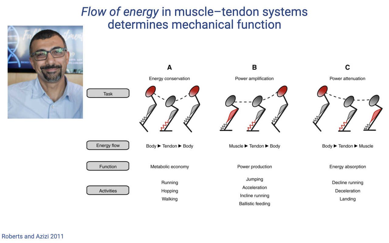
Three Energy-Flow Roles for Muscle–Tendon Units
- Roberts and Azizi (2011) classify muscle–tendon function by direction of energy flow through the system — a complementary view to the motor/strut/brake classification.
- A — Energy conservation (Body ► Tendon ► Body):
- Body kinetic and gravitational energy is stretched into the tendon, then returned to the body during push-off.
- Muscle acts as a near-isometric strut, allowing the tendon to cycle elastically.
- Function: metabolic economy. Activities: running, hopping, walking.
- B — Power amplification (Muscle ► Tendon ► Body):
- Muscle contracts (often slowly) and loads the tendon with energy; the tendon then releases that energy rapidly to the body.
- The tendon acts as a biological catapult, multiplying the muscle’s peak power output.
- Function: power production. Activities: jumping, acceleration, incline running, ballistic feeding (e.g., frog tongue, mantis shrimp strike).
- C — Power attenuation (Body ► Tendon ► Muscle):
- Body energy is absorbed by stretching the tendon, which then dissipates that energy by lengthening the active muscle.
- Muscle acts as a brake doing negative work; the tendon smooths the loading rate so the muscle is not torn.
- Function: energy absorption. Activities: decline running, deceleration, landing.
- Take-home: the same muscle–tendon unit can serve any of these three roles by changing the relative timing of muscle activation, body motion, and tendon stretch. The work-loop framework (Slides 5–6) is the mechanical fingerprint of which role is being played.
Slide 8
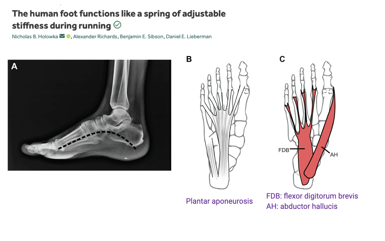
The Human Foot as an Adjustable Spring (Set-up)
- The longitudinal plantar arch is supported by a passive plantar aponeurosis and several intrinsic foot muscles — notably flexor digitorum brevis (FDB) and abductor hallucis (AH).
- The plantar aponeurosis behaves as a passive elastic element — stretched at midstance as the arch flattens under load, then recoils at push-off to return energy.
- The intrinsic muscles (FDB, AH) lie in parallel with the aponeurosis. Their activation level can effectively change the stiffness of the spring complex — making the foot stiffer when more muscle is co-activated, more compliant when less.
- The hypothesis Holowka et al. test: rather than being a fixed passive spring, the human arch is an actively tunable spring whose stiffness is set by the intrinsic muscles to match the demand of the task (e.g., stride frequency).
Slide 9
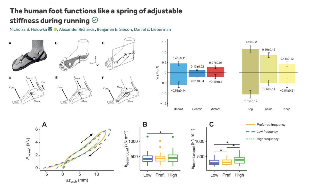
Foot Stiffness Is Tuned to Stride Frequency
- Mechanical framework (panels A–F): the foot is treated as a coupled beam-bending structure — Beam1 (forefoot), Beam2 (midfoot), and the midfoot arch act as elastic elements that absorb and return energy at each step.
- Top-right bar plots: each foot segment stores and returns measurable mechanical work each stride; the magnitudes are comparable to (though smaller than) those of the leg, ankle, and knee.
- Bottom-left work loops (Fbeam1 vs. Δzarch):
- Each loop is roughly elliptical with a clockwise sense — consistent with elastic spring behavior with a modest hysteresis loss.
- The three loops (low, preferred, high stride frequency) overlap in shape but differ in slope (stiffness).
- Bottom-middle and bottom-right box plots:
- Loading stiffness (kbeam1,load): significantly different across frequencies (asterisk marked).
- Unloading stiffness (kbeam1,unload): differs across all three pairwise comparisons (three asterisks) — high-frequency running produces the highest foot stiffness, low-frequency running the lowest.
- Key finding: arch stiffness is not a fixed property of the foot’s passive anatomy. The CNS adjusts intrinsic-muscle co-activation to match foot stiffness to stride frequency — exactly the prediction of the adjustable-spring model on Slide 8.
- Connects directly back to the work-loop framework: the arch is the textbook example of a near-elastic, slightly hysteretic spring, and the foot’s intrinsic muscles play a tuning role analogous to the soleus tuning the Achilles in Lecture 14.
Slide 10
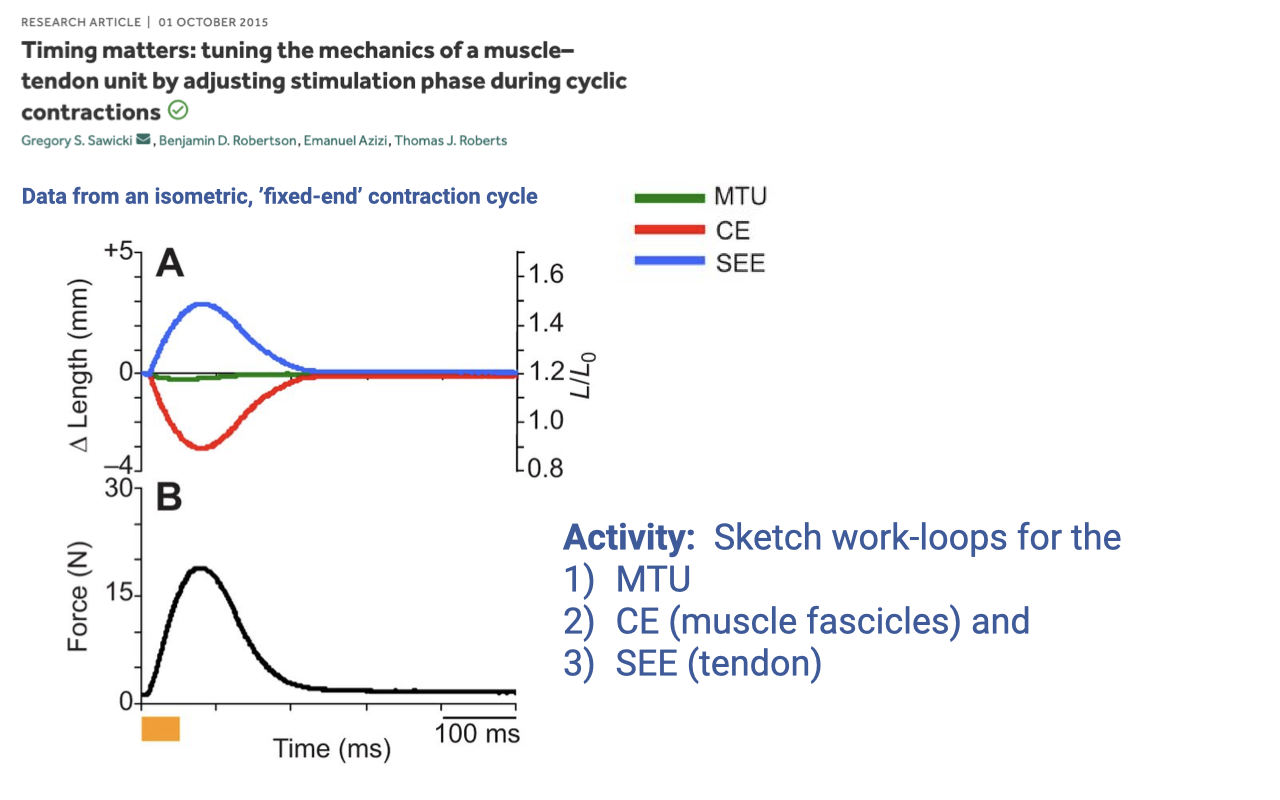
Activity 1 — Sketch Work Loops for an Isometric, Fixed-End Contraction
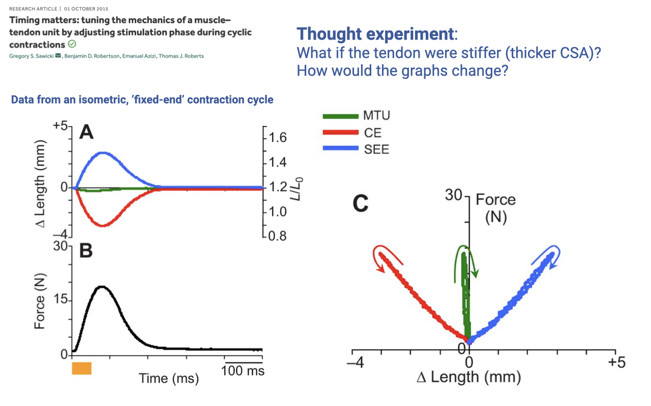
- Set-up (Sawicki et al. 2015): the whole muscle–tendon unit (MTU) is held at fixed end-to-end length. When the muscle is stimulated:
- MTU length (green) stays essentially flat at zero — the external ends do not move.
- CE (contractile element / fascicle, red) shortens by ~3 mm — the muscle pulls on the tendon.
- SEE (series elastic element / tendon, blue) stretches by ~+3 mm — equal and opposite to CE shortening so the MTU length is conserved.
- Force (Panel B) rises and falls as a single pulse over ~100 ms.
- Activity: sketch the predicted F–L work-loop shape for each of the three elements — MTU, CE, and SEE — using the time-domain traces above. The answer is shown on Slide 11.
Slide 11
Activity 1 — Answer and Thought Experiment
- Expected work-loop shapes (Panel C):
- MTU loop (green) — length is constant, so the F–L “loop” collapses to a vertical line at ΔLMTU ≈ 0. No enclosed area → no net MTU work.
- SEE loop (blue) — narrow, clockwise loop on the positive Δ-length side (tendon stretched to about +3 mm). The loop is nearly springlike; the small enclosed area is a slightly negative work loop reflecting modest elastic hysteresis. The tendon absorbs energy during stretch and returns most of it during recoil, with a small amount of energy lost as heat.
- CE loop (red) — counterclockwise loop on the negative Δ-length side (muscle shortened to about −3 mm). The direction of the trace is the exact reflected version of the SEE loop. The enclosed area is nearly zero because no net work is done over the cycle (the MTU end-points are fixed). The small enclosed area corresponds to a very small amount of positive muscle work, exactly equal to the hysteresis energy lost in the tendon — the muscle is the active source of that small make-up energy.
- Energy bookkeeping: the muscle does positive work early, the tendon stores and returns most of it, and the MTU end-points do no external work over the complete cycle. The whole exchange is internal — muscle → tendon → muscle.
- Thought experiment — stiffer tendon (larger CSA):
- For the same muscle force, a stiffer tendon stretches less (F = k·Δx with larger k → smaller Δx).
- Because the MTU length is fixed, the muscle must shorten less as well — the red CE loop shrinks to a smaller Δ-length range.
- The blue SEE loop also narrows along the Δ-length axis.
- The muscle ends up operating closer to isometric — at a length where its force capacity may be higher, but at the cost of lower elastic energy cycling in the tendon.
- Conceptual link: tendon stiffness is a design parameter that influences muscle-tendon function. Optimal stiffness depends on the task — too stiff and elastic energy is not stored in the tendon, but the muscle directly actuates the joint; too compliant and the muscle mostly does work stretching the tendon without moving the joint.
Slide 12
Activity 2 — Sketch Work Loops for Cyclic Contractions
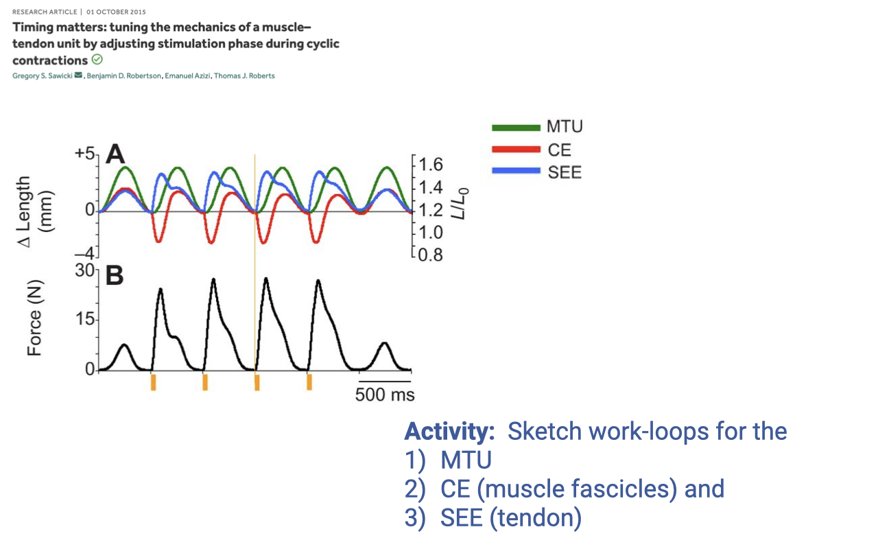
- Set-up: same Sawicki et al. preparation as in Activity 1, but now the MTU is driven through a cyclic length trajectory (sinusoidal length change), with one stimulation pulse per cycle delivered near the start of the lengthening phase.
- Reading the panels (before sketching):
- MTU (green) — sinusoidal length change between ~+4 and ~−4 mm; large external excursion at each cycle.
- CE (red, fascicle) — also oscillates, but with different phasing than the MTU; stretches during the rising-force phase.
- SEE (blue, tendon) — stretches and recoils
- Force (Panel B) — rises and falls as a train of pulses, one per cycle.
- Activity: sketch the predicted F–L work-loop shape for each of the three elements — MTU, CE, and SEE — using the time-domain traces above. The answer is shown on Slide 13.
Slide 13
Activity 2 — Answer for Cyclic Contractions
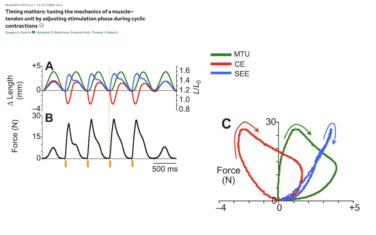
- Expected work-loop shapes (Panel C):
- MTU loop (green) — broad, clockwise loop in the positive-length region with substantial enclosed area → the MTU does net negative work (absorbs energy) from the external load.
- CE loop (red) — leftward-shifted, clockwise loop. The muscle absorbs net energy over the cycle.
- SEE loop (blue) — narrow, nearly springlike clockwise loop on the positive Δ-length side with very little enclosed area → near-elastic tendon behavior, with a small slightly negative area equal to the hysteresis loss.
- Why the loops differ from the fixed-end case: the MTU is no longer pinned at one length. The muscle is stretched during force development, and the MTU also stretches — so the MTU and CE loops are open with net area associated with net negative work.
- Big-picture take-away: in cyclic contractions, the MTU work loop is the net visible behavior at the joint, while the CE and SEE loops show how the active and passive elements share the load internally. The sign and shape of all three loops depend on when the muscle is activated relative to length change — the same preparation can produce positive (motor), near-zero (strut/spring), or negative (brake) net work at the MTU level just by shifting activation timing.
Key Equations
| Equation | Name | Description |
|---|---|---|
| $W = \oint F \, dL$ | Work loop (net mechanical work) | Net work over one cycle equals the enclosed area of the force–length trajectory. Sign is set by the direction of travel: counterclockwise → positive (motor), clockwise → negative (brake), zero enclosed area → strut/spring. |
| $L_{\text{MTU}} = L_{\text{CE}} + L_{\text{SEE}}$ | Muscle-tendon unit length partition | At every instant, MTU length equals the sum of contractile-element (fascicle) length and series-elastic-element (tendon) length. For a fixed-end contraction $\Delta L_{\text{MTU}} = 0$, so any fascicle shortening must equal tendon stretch. |
| $F_{\text{CE}} = F_{\text{SEE}}$ | Series-element force balance | In a series CE–SEE arrangement, the contractile element and tendon transmit the same force at every instant. |
| $F_{\text{SEE}} = k_{\text{tendon}} \cdot \Delta L_{\text{SEE}}$ | Tendon stiffness relationship | Tendon force is approximately linear in tendon stretch over the operating range; stiffness k increases with tendon cross-sectional area (Slide 11 thought experiment). |
Glossary of Key Terms
| Term | Definition |
|---|---|
| Exercise-associated muscle cramps (EAMC) | Painful, involuntary, sustained muscle contractions during or just after exercise. Best-supported mechanism is altered neuromuscular control (fatigue-driven hyperexcitability of α-motor neurons), not dehydration or electrolyte loss. |
| Older (dehydration/electrolyte) model of cramps | Historical model attributing EAMC to sweat-driven losses of plasma Na+ and extracellular fluid. Not supported by prospective cohort data: serum electrolytes and hydration status are similar in crampers and non-crampers. |
| Current (neuromuscular control) model of cramps | Model in which muscle fatigue increases muscle-spindle (Ia) drive and decreases Golgi-tendon-organ (Ib) inhibition, producing hyperexcitable α-motor neurons. Predicts localized cramping in working, shortened muscles and relief by stretch. |
| Oropharyngeal reflex | Sensory pathway by which strong tastes (vinegar in pickle juice) activate receptors in the mouth and pharynx that send inhibitory signals to spinal α-motor neurons — the proposed mechanism for pickle-juice-induced cramp relief. |
| PubMed indexing | A quality filter: a journal indexed in the NIH PubMed database has met basic editorial standards. Google Scholar indexes far more broadly and does not filter by journal quality. |
| Systematic review and meta-analysis | A review that uses keyword searches to find all papers on a topic, applies quality filters, and synthesizes the evidence statistically. Considered the gold standard because it integrates across many studies and reduces single-study bias. |
| Work loop | Plot of muscle force vs. muscle length over one contraction cycle. The enclosed area is the net mechanical work; the direction of travel sets the sign. Standard graphical tool for classifying muscle function as motor, strut/spring, or brake. |
| MTU (muscle-tendon unit) | The whole functional unit from one tendinous attachment to the other, including the contractile element (muscle fibers) and the series elastic element (tendon and aponeurosis). |
| CE (contractile element) | The active, cross-bridge-cycling component of the MTU — i.e., the muscle fascicles. Source of active force generation and the only part of the MTU that consumes metabolic energy. |
| SEE (series elastic element) | The passive elastic component in series with the CE — primarily the tendon, plus the aponeurosis. Stretches when force rises and recoils when force falls; cycles energy elastically. |
| Energy conservation (Roberts & Azizi A) | Energy flow Body ► Tendon ► Body. Muscle near-isometric; tendon stores and returns body energy; produces metabolic economy. Activities: walking, running, hopping. |
| Power amplification (Roberts & Azizi B) | Energy flow Muscle ► Tendon ► Body. Muscle loads the tendon slowly; tendon releases energy rapidly; produces a power burst. Activities: jumping, acceleration, incline running, ballistic feeding. |
| Power attenuation (Roberts & Azizi C) | Energy flow Body ► Tendon ► Muscle. Tendon absorbs body energy; muscle dissipates it by lengthening under load. Activities: decline running, deceleration, landing. |
| Plantar aponeurosis | The passive elastic sheet running from the calcaneus to the toe pads, supporting the longitudinal arch of the human foot and acting as the foot’s principal series elastic element. |
| Intrinsic foot muscles (FDB, AH) | Flexor digitorum brevis and abductor hallucis are short intrinsic muscles of the plantar foot that lie in parallel with the plantar aponeurosis and adjust foot stiffness by changing their co-activation. |
| Adjustable stiffness (foot) | Property of the human foot in which activation of intrinsic muscles tunes the stiffness of the arch spring. Holowka et al. show arch stiffness rises with stride frequency, consistent with active tuning of the elastic system. |