Lecture 14: Integrative Muscle Function 4 — Limb and Whole-Organism Level
Slide 1
- Final lecture in the muscle structure-and-function sequence — moving from the organ and limb scales of Lecture 13 up to the whole-organism scale of muscle function during locomotion.
- Continues the central theme: trade-offs at every structural level integrate to determine how muscles actually work in real movement.
- Today connects the intrinsic properties (Lecture 12) and architecture/lever systems (Lecture 13) to direct measurements of muscle function during locomotion in animals and humans.
Slide 2
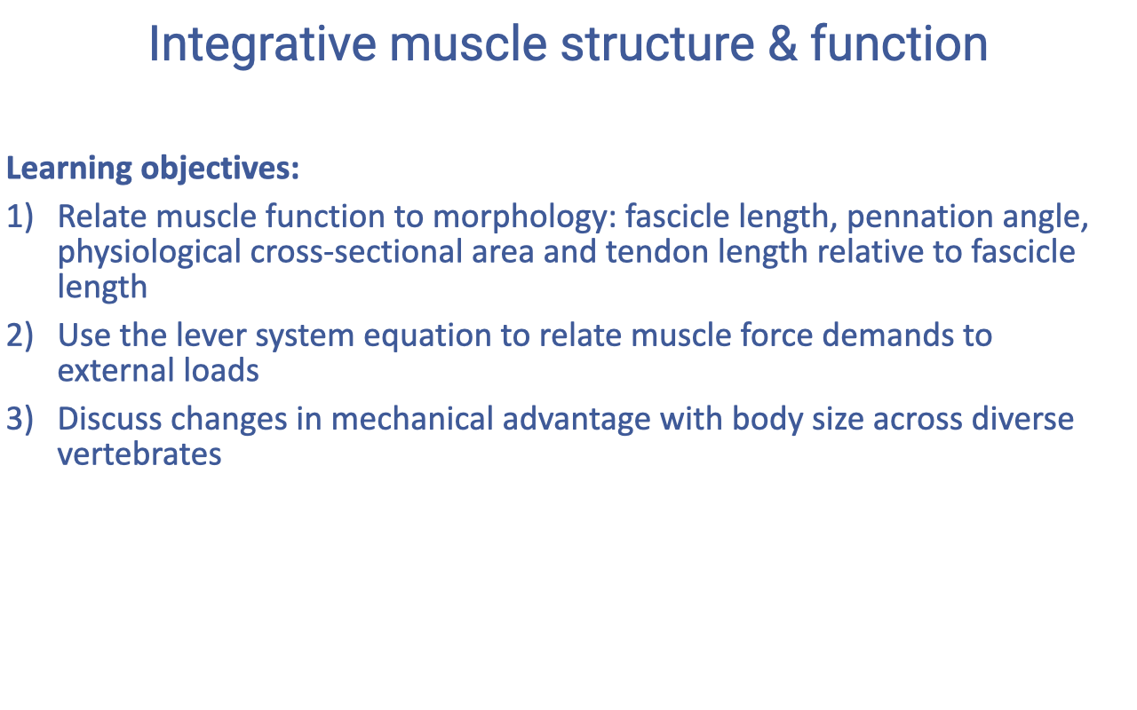
Recap — Lecture 13 Learning Objectives
- Recap of last lecture’s three objectives:
- Relate muscle function to morphology: fascicle length, pennation angle, PCSA, and tendon length relative to fascicle length.
- Use the lever-system equation to relate muscle-force demands to externally applied loads.
- Discuss how effective mechanical advantage (EMA) scales with body size across diverse vertebrates.
- These set the foundation for today’s integrative content.
Slide 3
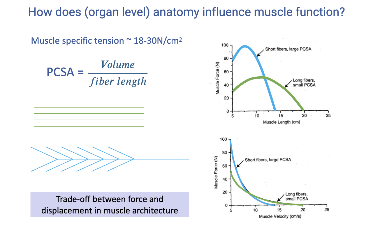
Recap — Architectural Force–Length and Force–Velocity Trade-offs
- Specific tension ~18–30 N/cm² (highly conserved across vertebrates).
- Physiological cross-sectional area: $\text{PCSA} = \text{Volume} / L_{fiber}$.
- The architectural trade-off at the muscle–tendon unit level:
- Short fibers, large PCSA → high peak force, narrow operating range, lower Vmax.
- Long fibers, small PCSA → lower peak force, wider operating range, higher Vmax.
- This MTU-level trade-off is independent of fiber type — both come from the architecture of the muscle.
Slide 4
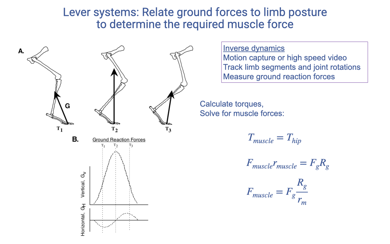
Recap — Limb Lever Systems and Inverse Dynamics
- Inverse dynamics uses external measurements (motion capture / high-speed video; ground reaction force) to infer internal muscle forces.
- At each joint, the torque balance gives:
- rm (muscle moment arm) is set by skeletal morphology.
- Rg (GRF moment arm) is set by limb posture during the gait cycle.
- This technique is the workhorse of musculoskeletal biomechanics — it lets researchers estimate muscle and joint loads non-invasively.
Slide 5
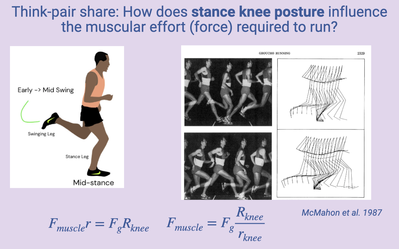
Class Activity — Stance Knee Posture and Muscular Effort
- Think-pair-share prompt: how does stance-knee posture influence the muscular effort required to run?
- McMahon et al. 1987 classic study: compared normal upright running with “Groucho running” (deliberately flexed knees).
- Lever-system reasoning:
- More flexed knee → ground reaction force vector falls further from the knee joint center.
- Rknee increases → muscle force Fmuscle = Fg × Rknee / rknee increases.
- Crouched running requires greater quadriceps force for the same ground reaction force.
- Why one might still crouch:
- Jumping — larger angular excursion stores and releases more energy.
- Running downhill — eccentric contractions can generate large forces economically.
- Uneven terrain — a more compliant, crouched limb absorbs perturbations and is more stable than a stiff straight limb. Trade-off between economy and stability.
Slide 6
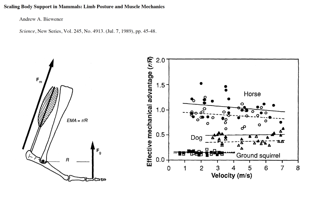
Recap — EMA and the Biewener Scaling Result
- The effective mechanical advantage EMA = r/R.
- Across species (horse, dog, ground squirrel), EMA is roughly constant with running velocity within a species, but shifts dramatically with body size between species.
- The mechanism is a postural shift with body size — small animals adopt crouched postures; large animals stand more upright.
Slide 7
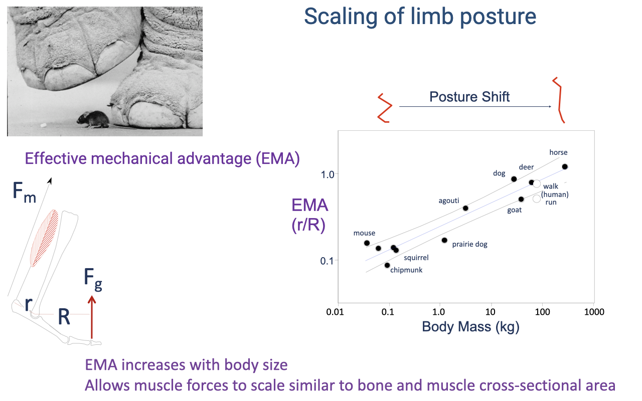
Recap — EMA Scales With Body Mass
- EMA scales positively with body mass across mammals (mouse → horse).
- Muscle (and bone) forces scale similarly to muscle (and bone) cross-sectional area — preventing large animals from breaking under their own weight.
- Without this postural scaling, an elephant-sized animal would need impossibly proportionally massive muscles and bones to support its weight.
Slide 8
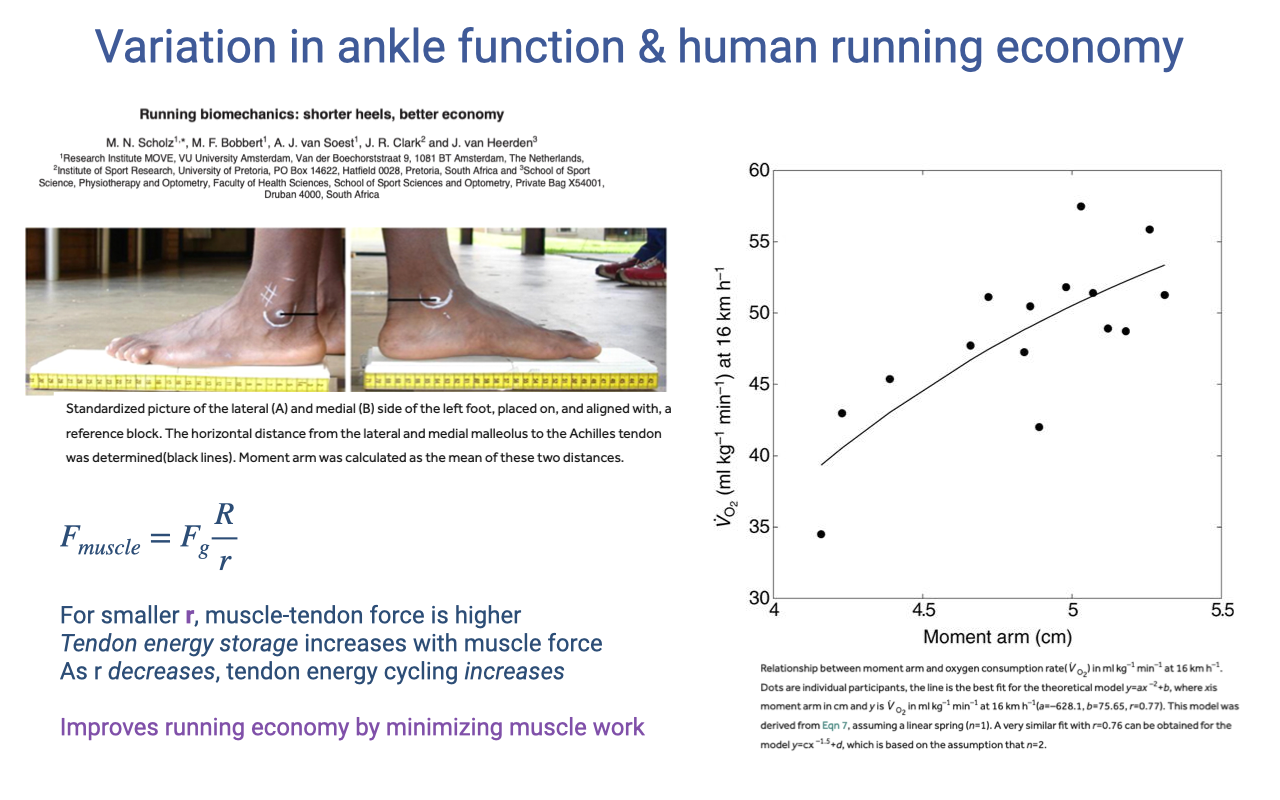
Recap — Ankle Moment Arm and Running Economy
- Within humans, shorter ankle moment arm (r) → better running economy.
- Mechanism is counterintuitive but important for today:
- Smaller r → higher muscle–tendon force from the lever equation.
- But higher force → more tendon strain energy storage.
- The tendon’s elastic energy cycling does work the muscle would otherwise have to do — improving economy.
- This is the bridge into today’s lecture: muscle, tendon, and skeletal lever systems work together to produce real in vivo function.
Slide 9
Today’s Learning Objectives
- Describe how muscles function during cyclical contractions using examples from comparative and human studies.
- Sketch a cyclical muscle work-loop for a muscle that produces power and a muscle that cycles elastic energy.
- Discuss the role of tendon in cyclical (steady-state), power-producing, and energy-absorbing tasks.
- Today’s content provides the foundation for next week’s material on metabolic energy cost of locomotion.
Slide 10
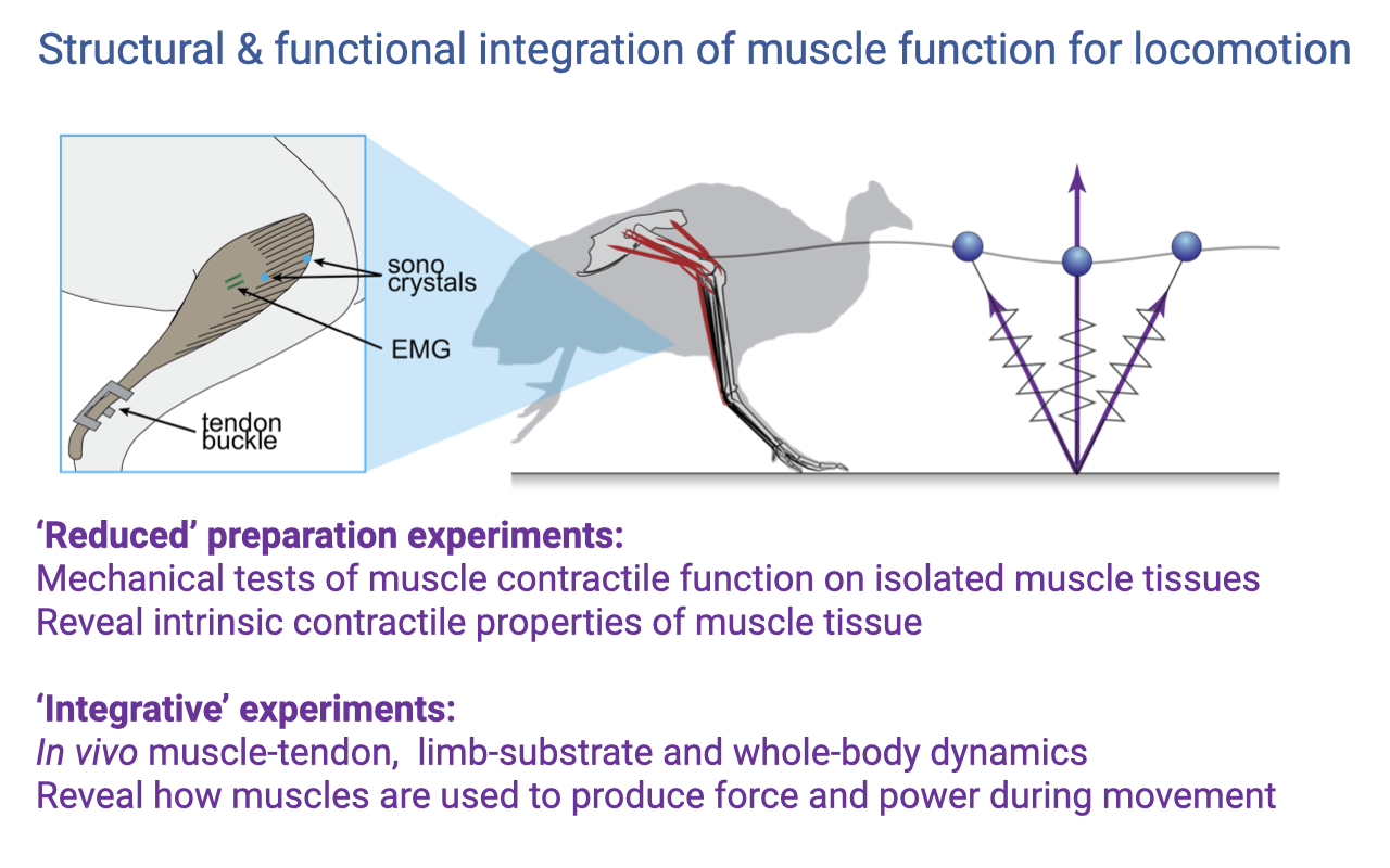
Two Categories of Experiments
- Reduced preparation experiments (Lectures 11–12):
- Isolated muscle on a bench-top apparatus.
- Reveal intrinsic contractile properties (F–L, F–V, activation).
- Integrative experiments (today):
- In vivo muscle–tendon, limb–substrate, and whole-body dynamics.
- Reveal how muscles are actually used during real movement.
- Both approaches are needed — intrinsic properties define what the muscle is capable of; integrative experiments reveal what it actually does within the integrated system.
Slide 11
Transition — From Intrinsic Properties to In Vivo Function
- Transition slide motivating the central question of the lecture: how do intrinsic properties and anatomy combine to determine muscle function in locomotion?
- Sets up the next section, which surveys comparative anatomical patterns in cursorial limbs and the direct measurements that connect those patterns to function.
Slide 12
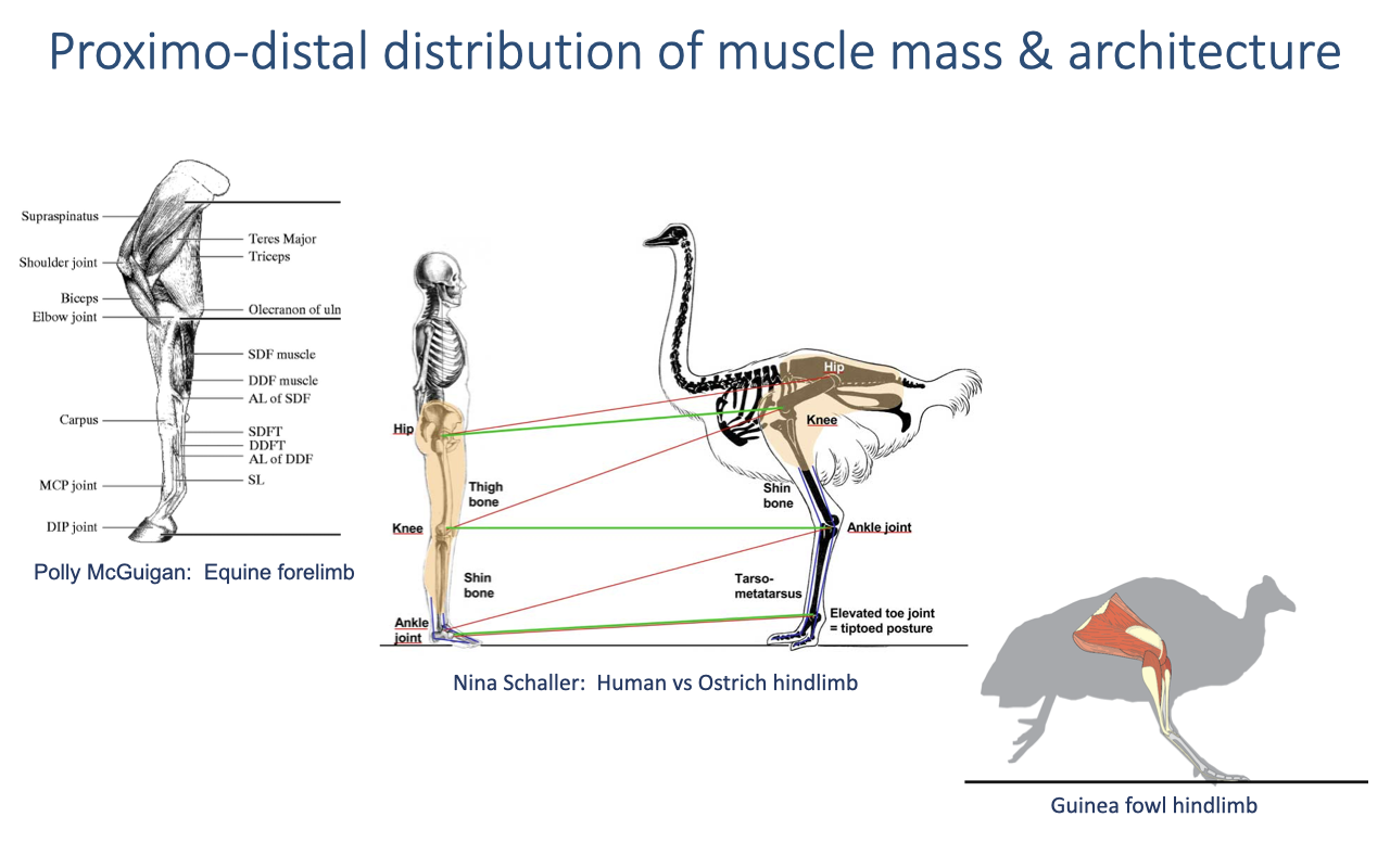
Proximo-Distal Architectural Gradient
- Comparative observation across cursorial vertebrates (horses, ostriches, guinea fowl, humans, dogs, etc.):
- Proximal joints (hip, shoulder): large-mass muscles with long fibers and short tendons — designed for high work and power.
- Distal joints (ankle, wrist): small-mass muscles with short fibers and very long tendons — designed for economy and elastic energy cycling.
- Extreme examples:
- Horse forelimb: distal limb is almost entirely tendon and ligament; muscle mass is concentrated proximally.
- Ostrich hindlimb: very long, highly tendinous distal segment; massive proximal muscles.
- Humans are unusual: relatively heavy distal limbs (calf muscles + foot are non-trivial mass) compared to specialized cursorial animals.
Slide 13
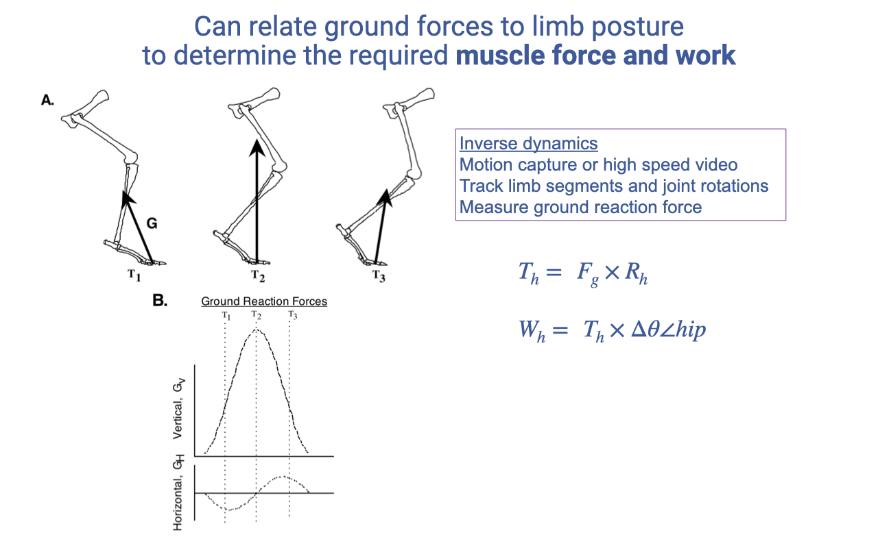
Inverse Dynamics — Joint Torques and Work
- Inverse dynamics workflow:
- Capture motion (motion capture or high-speed video) and ground reaction forces.
- Track limb segments and joint rotations through the stance phase.
- Compute joint torque at each joint: $T_h = F_g \times R_h$.
- Compute joint work by integrating torque × angular displacement: $W_h = T_h \times \Delta\theta_{hip}$.
- Net joint work (positive or negative) reveals which joints are producing energy, absorbing energy, or operating isometrically.
Slide 14
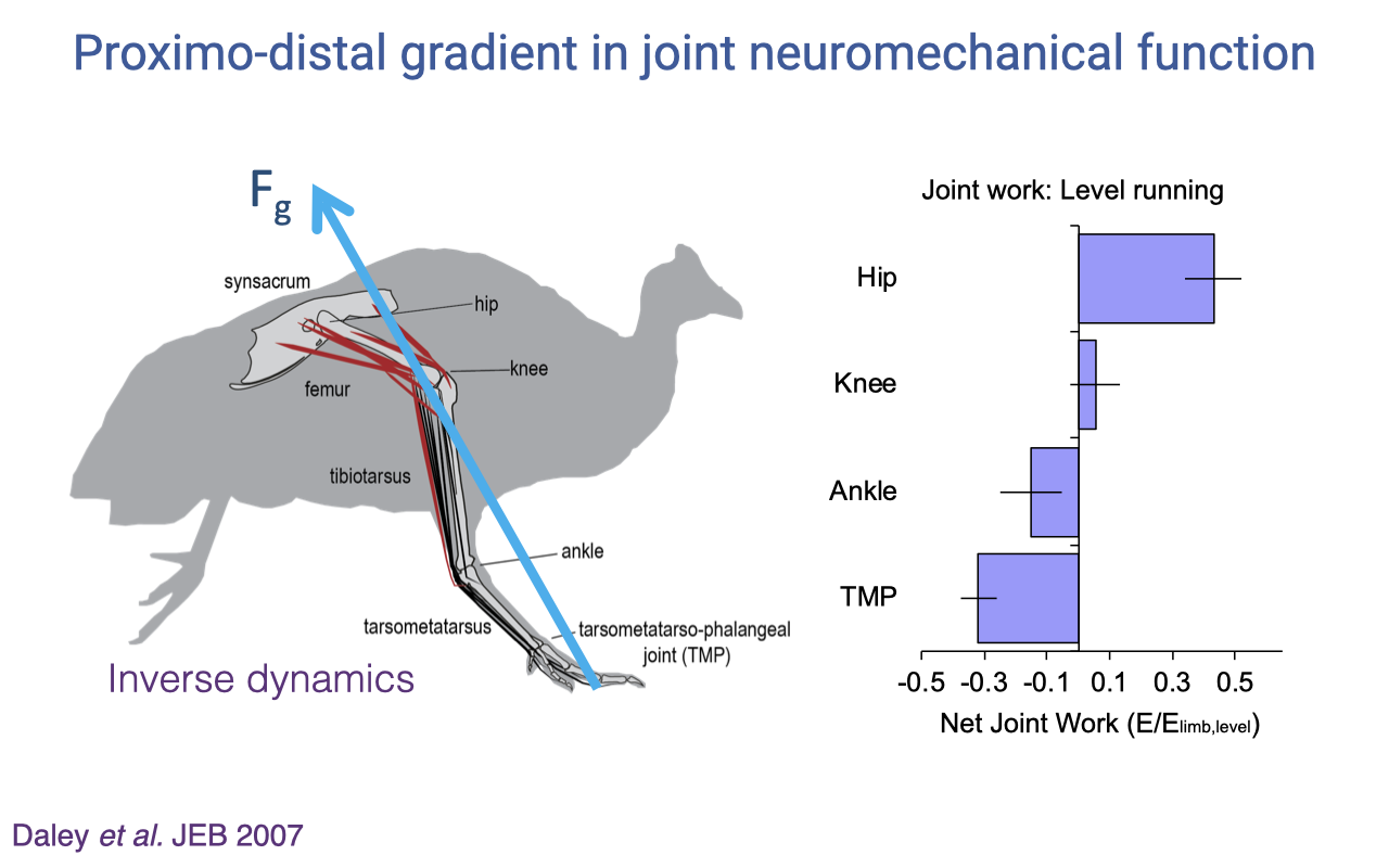
Proximo-Distal Gradient in Joint Function — Daley et al. 2007
- Inverse-dynamics analysis of the guinea fowl hindlimb (Daley et al. 2007 JEB):
- Hip: produces large positive net work (energy generation — power production).
- Knee: small net work, near isometric.
- Ankle: small negative net work (energy absorption / spring-like cycling).
- Tarsometatarso-phalangeal (TMP): large negative net work (energy absorption).
- This gradient maps directly onto the architectural gradient from Slide 12:
- Power-producing proximal joints are driven by muscles with long fibers and short tendons (high work capacity).
- Energy-absorbing or spring-like distal joints are driven by muscles with short fibers and long tendons (high elastic-cycling capacity).
Slide 15
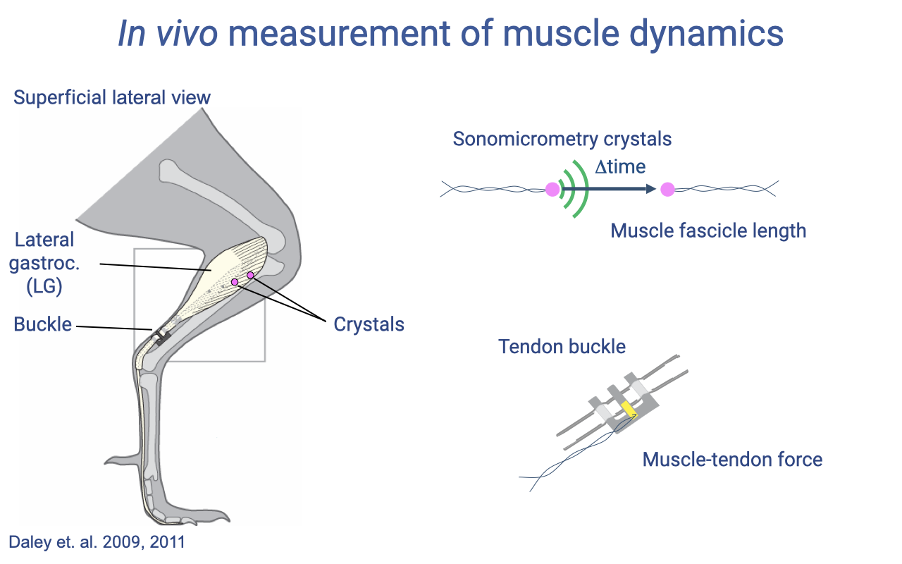
In Vivo Measurement Tools — Sonomicrometry and Tendon Buckles
- Sonomicrometry crystals: pairs of small piezoelectric crystals implanted in the muscle. They emit and receive ultrasonic pulses, and the time of flight between them gives muscle fascicle length with sub-millisecond resolution.
- Tendon buckle: a small strain-gauge transducer surgically attached to the tendon; deformation of the buckle by tendon force is converted to a force signal — yielding direct in vivo muscle–tendon force.
- EMG electrodes (Slide 10) record the timing of activation.
- Together, these tools provide simultaneous length, force, and activation measurements during real movement — the direct equivalent of the lab F–L and F–V experiments, but in the moving animal.
Slide 16
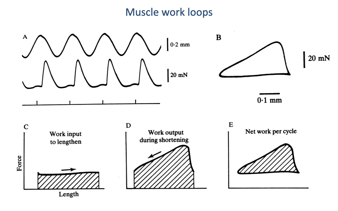
Muscle Work Loops — A Tool for Visualizing Energy Flow
- A work loop plots force vs. length through one complete cycle of contraction. The area enclosed is the net mechanical work per cycle.
- Counterclockwise loop (force higher during shortening than during lengthening) → net positive work — the muscle is acting as a motor.
- Clockwise loop (force higher during lengthening than during shortening) → net negative work — the muscle is acting as a brake (energy absorber).
- A narrow, flat loop with little enclosed area → muscle is acting near-isometrically — operating like a spring or strut, with most of the energy cycling through the tendon rather than through cross-bridge cycling.
Slide 17
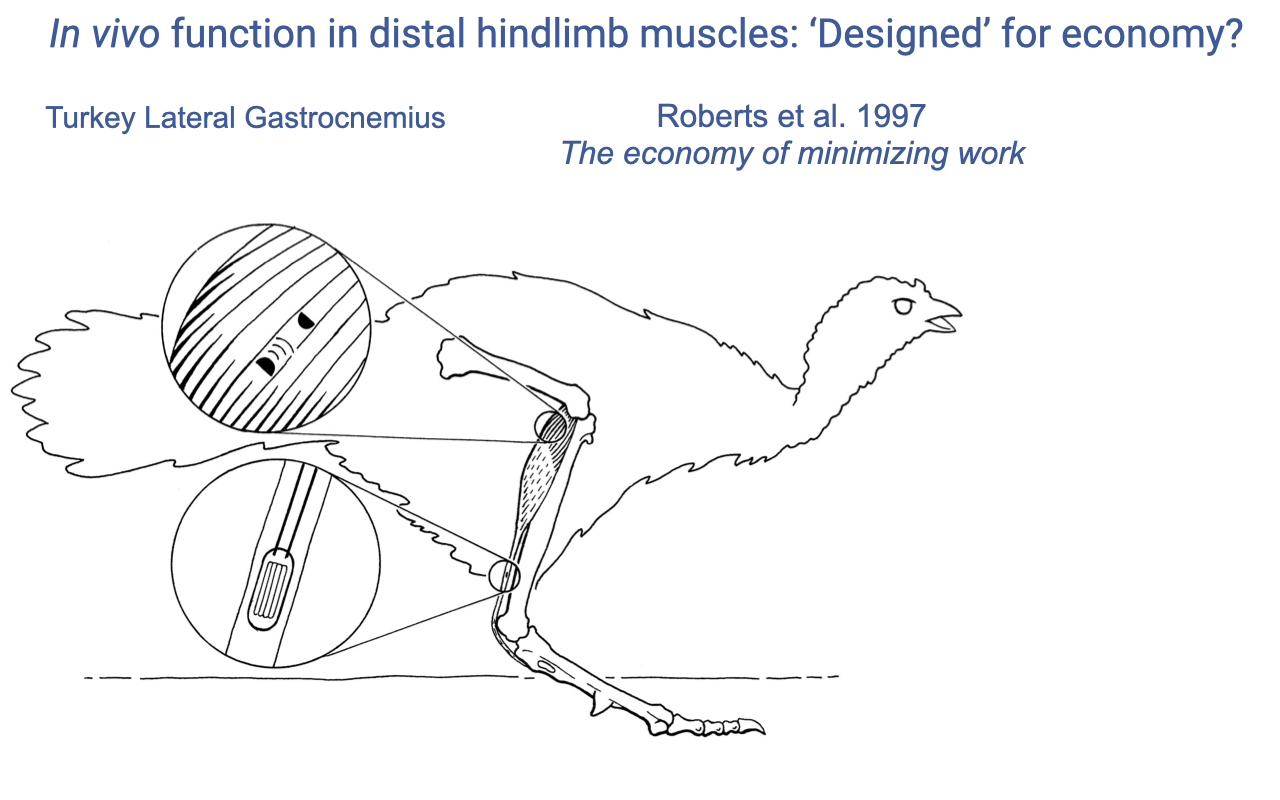
Roberts et al. 1997 — Turkey Lateral Gastrocnemius
- Roberts et al. 1997 Science — landmark paper: “Muscular force in running turkeys: the economy of minimizing work.”
- Methodology:
- Sonomicrometry crystals in the lateral gastrocnemius (LG) — measure fascicle length.
- Tendon buckle on the Achilles tendon — measure muscle–tendon force.
- EMG — measure activation timing.
- This is the prototype experiment for in vivo muscle dynamics in cursorial locomotion.
Slide 18
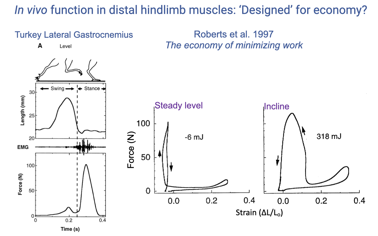
Turkey LG — Level vs. Incline Running
- Two iconic Roberts et al. 1997 work loops:
- Level (steady) running: force–strain loop is tall and narrow, with near-zero net work (W ≈ −6 mJ per cycle).
- Muscle generates force at near-constant length — the tendon stretches and recoils.
- Muscle acts as a strut/spring with most of the work cycling through the tendon.
- Incline running (uphill): force–strain loop is wide, with substantial positive work (W ≈ +318 mJ per cycle).
- Muscle actively shortens under high force — performing positive work to lift the body against gravity.
- Muscle acts as a motor.
- Level (steady) running: force–strain loop is tall and narrow, with near-zero net work (W ≈ −6 mJ per cycle).
- The same muscle can produce dramatically different mechanical outputs depending on the task.
Slide 19
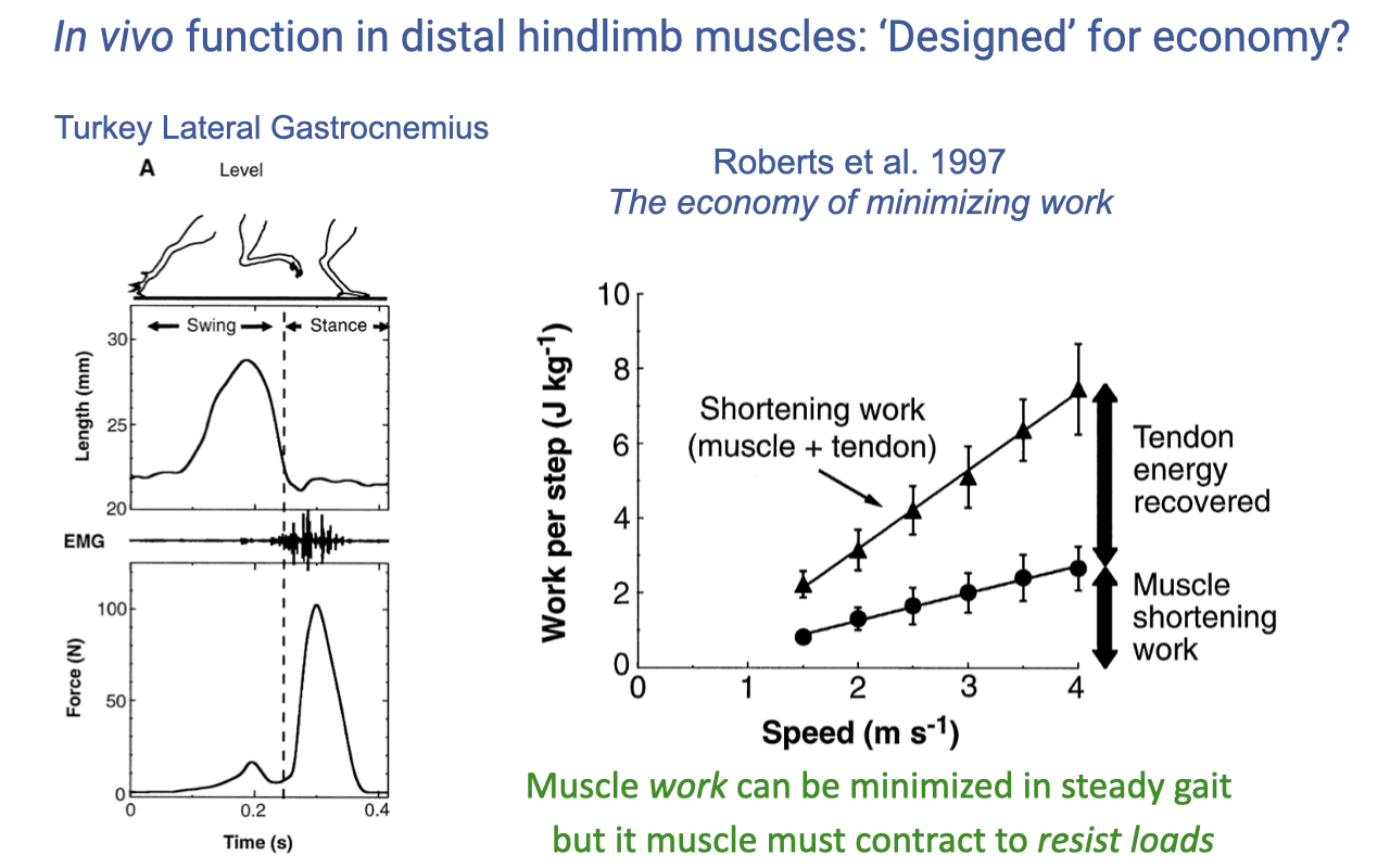
Tendon Energy Recovery in the Turkey LG
- During level running at all speeds, muscle shortening work is much less than total muscle–tendon shortening work:
- The difference is tendon strain energy that is stored on landing and recovered during the propulsive phase.
- Most of the work done by the muscle–tendon unit comes from the tendon spring, not the muscle’s contractile work.
- Muscle work can be minimized in steady gait, but the muscle must still contract isometrically to resist the loads that stretch the tendon. So the muscle still costs ATP, even when doing little mechanical work.
Slide 20
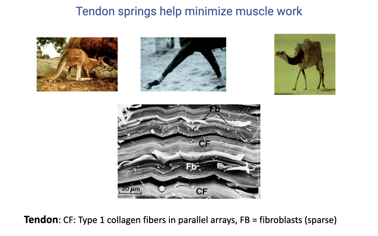
Why Tendons Are Excellent Springs
- Tendon is composed of Type I collagen fibers in highly aligned parallel arrays, with sparsely distributed fibroblasts between layers.
- This near-crystalline organization gives tendon:
- High tensile stiffness (large force capacity).
- High elastic energy storage (~95% energy return).
- Low metabolic cost (no active cellular work to store energy).
- Across vertebrates (kangaroos, runners, camels), distal-limb tendons act as passive springs — drastically reducing the metabolic cost of locomotion.
Slide 21
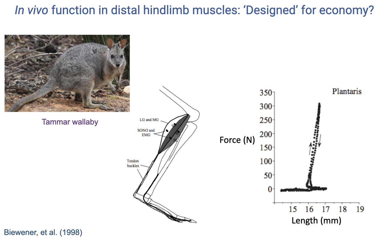
Wallaby Plantaris — Even More Spring-Like
- Biewener et al. (1998) measurements on the tammar wallaby plantaris:
- The force–length loop is even narrower than the turkey LG — almost a vertical line (300+ N at near-constant length).
- Plantaris fascicles barely change length during hopping — virtually all length change in the MTU is in the long, compliant Achilles tendon.
- In hopping marsupials, distal-limb muscles are extreme isometric force-generators; tendons do nearly all the mechanical work.
Slide 22
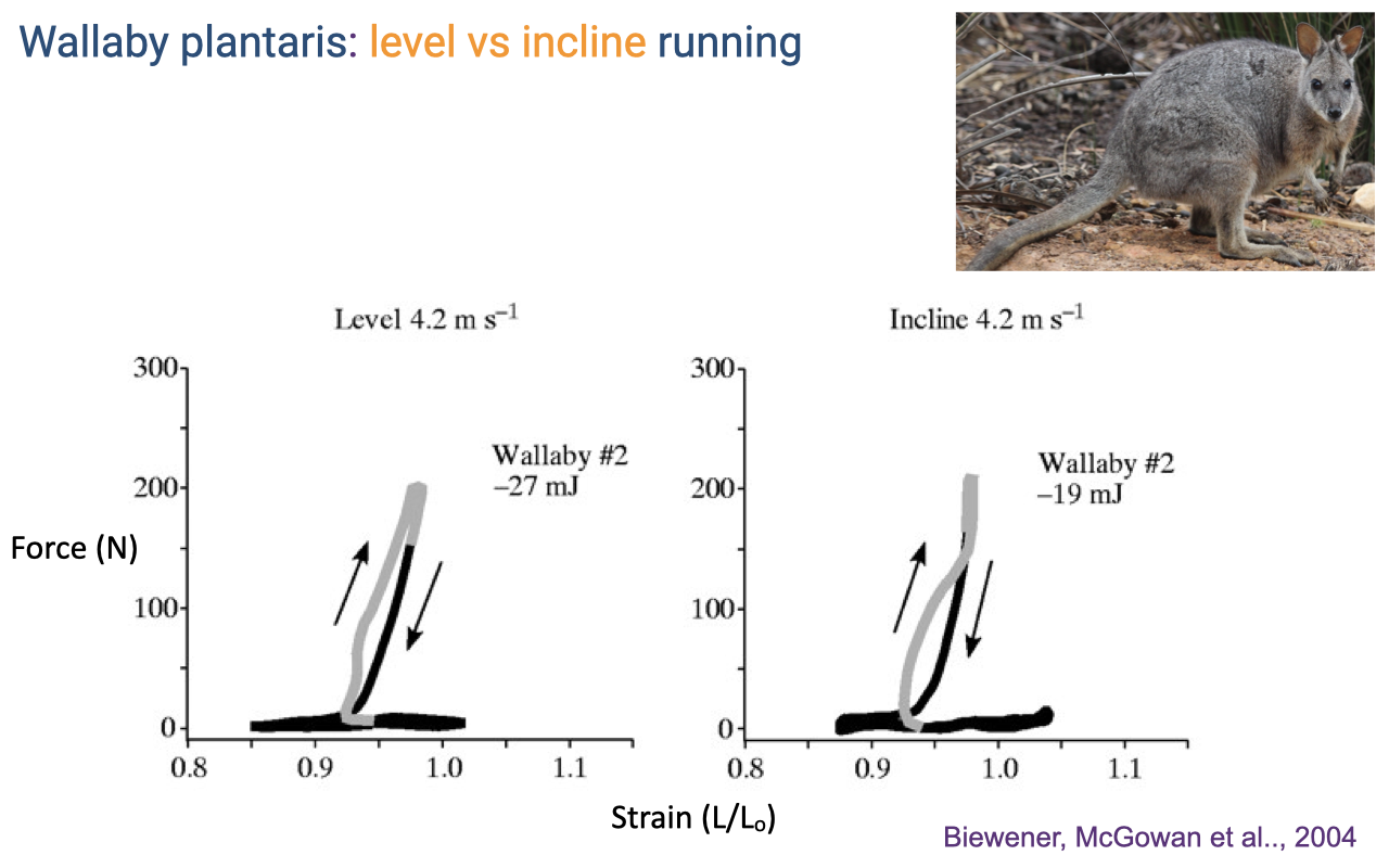
Wallaby Plantaris on Inclines
- Unlike the turkey LG (which shifts dramatically toward positive work on inclines), the wallaby plantaris retains a near-isometric loop on inclines (Biewener, McGowan et al. 2004).
- Net work changes only modestly (−27 mJ level → −19 mJ incline) — the muscle remains strut-like even when the animal is climbing.
- In wallabies, the proximal muscles (not the distal plantaris) take on the additional power-production task during incline locomotion.
Slide 23
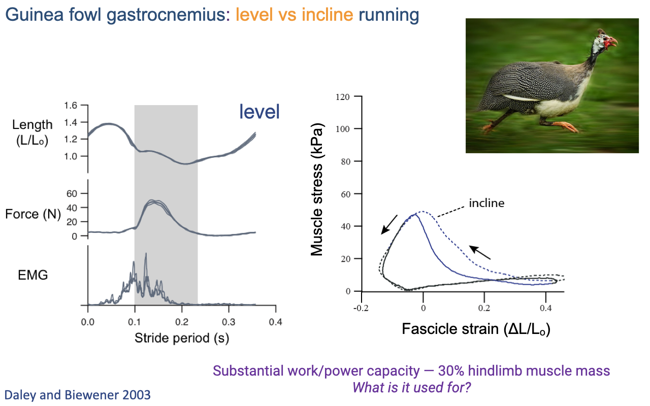
Guinea Fowl Lateral Gastrocnemius — Versatile Function
- Daley and Biewener 2003: guinea fowl LG behaves like turkey LG on level ground (mostly isometric, some shortening) and shifts to a much wider loop on inclines (substantial positive work).
- The LG comprises ~30% of total hindlimb muscle mass — a substantial work/power reservoir.
- Question for the next slide: if level running only requires near-isometric force, what is all that work capacity used for? Answer: non-steady tasks — accelerating, climbing, and stabilizing on uneven terrain.
Slide 24
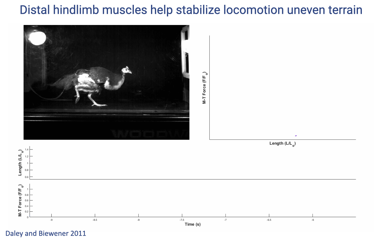
Distal Muscles Stabilize Locomotion on Uneven Terrain
- Daley and Biewener 2011: when guinea fowl run over uneven terrain, the LG modulates its work output stride-by-stride — sometimes acting as a strut, sometimes producing positive work, sometimes absorbing energy.
- This reserve work capacity explains the apparent “over-engineering” of the distal hindlimb muscles for level running.
- Provides autonomous mechanical stability through intrinsic muscle properties (force–length, force–velocity) — without requiring fast neural reflexes.
Slide 25
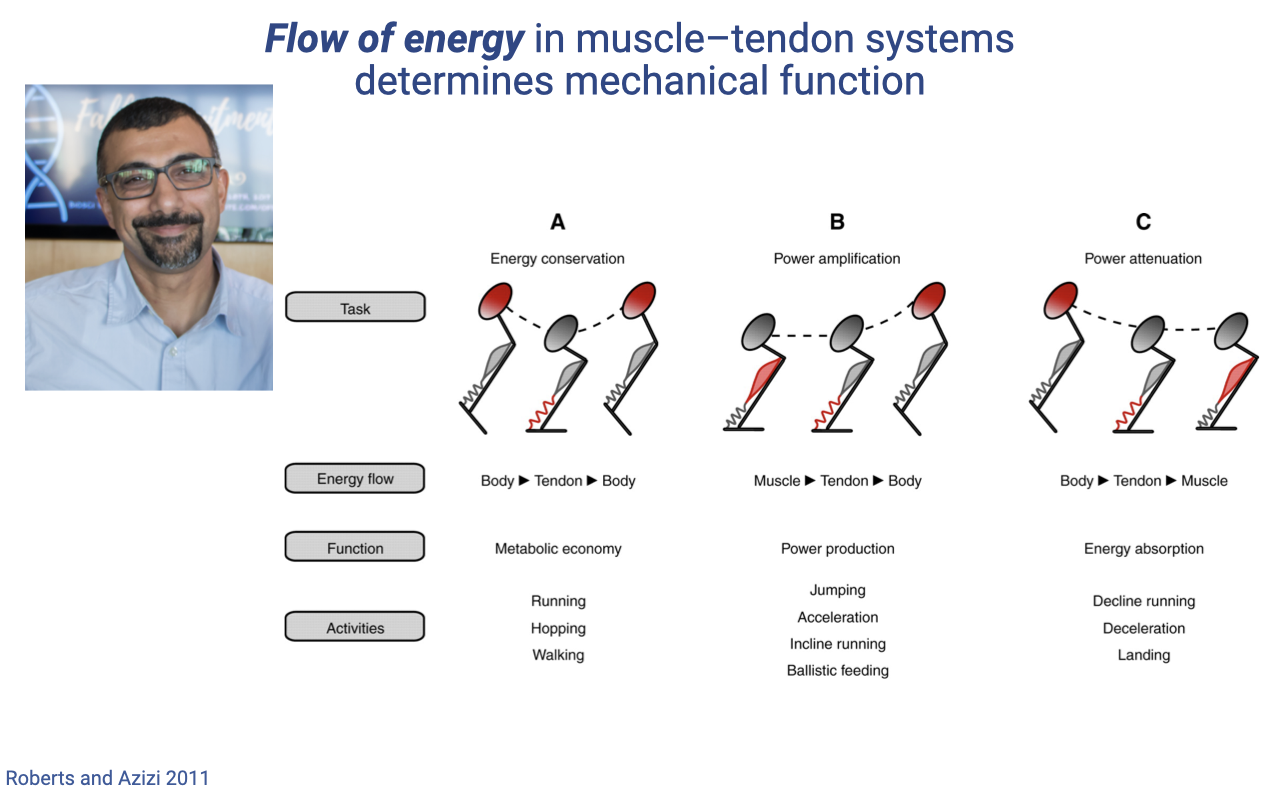
The Flow-of-Energy Framework — Roberts and Azizi 2011
| Mode | Energy flow | Muscle role | Function | Activities |
|---|---|---|---|---|
| (A) Energy conservation | Body → Tendon → Body | Strut (isometric) | Metabolic economy | Running, hopping, walking |
| (B) Power amplification | Muscle → Tendon → Body | Motor (concentric) | Power production | Jumping, acceleration, incline running, ballistic feeding |
| (C) Power attenuation | Body → Tendon → Muscle | Brake (eccentric) | Energy absorption | Decline running, deceleration, landing |
- The same muscle–tendon unit can switch between these modes depending on task demand and activation timing — a unifying framework for in vivo muscle function.
Slide 26
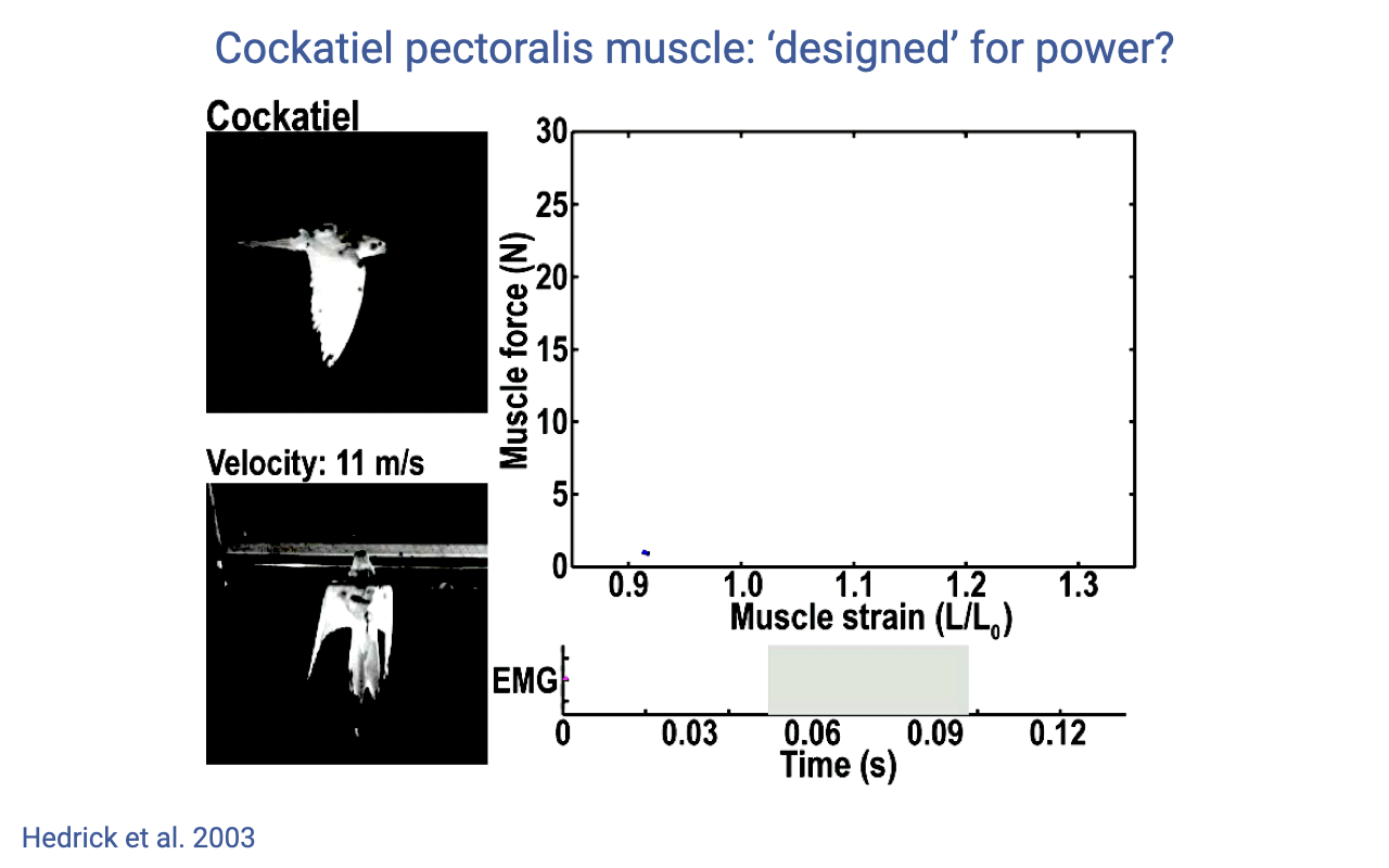
Cockatiel Pectoralis — A Pure Motor
- Hedrick et al. 2003: cockatiel pectoralis (downstroke flight muscle) during forward flight at 11 m/s.
- The work loop is wide and counterclockwise — large positive work per cycle.
- Pectoralis acts as a motor that produces all of the aerodynamic work needed for flight; the muscle shortens through a large strain range while generating force.
- Contrast with the turkey LG and wallaby plantaris (strut-like) — pectoralis is at the opposite end of the spectrum, dedicated entirely to power production.
Slide 27
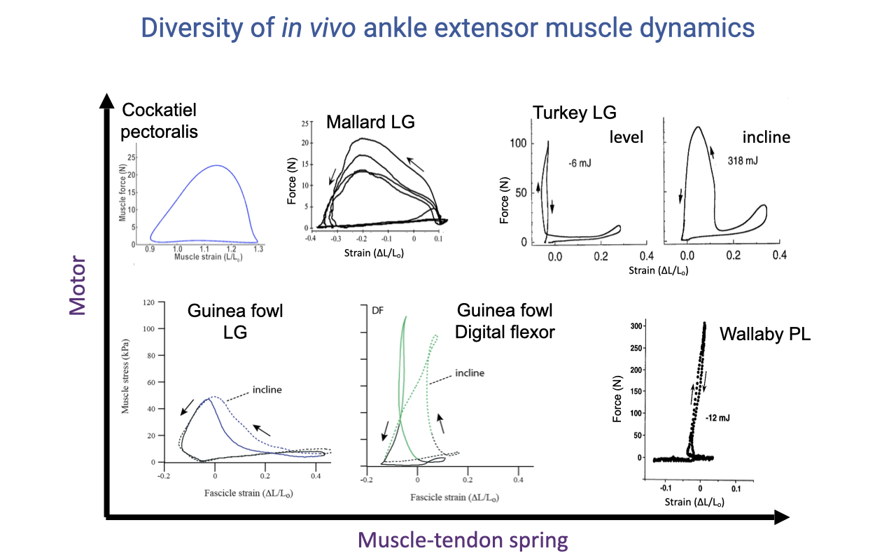
A Continuum from Motor to Spring
- A summary figure plotting many in vivo muscle work loops on a 2D space:
- Vertical axis (Motor): tall, wide loops with substantial positive work — high power output.
- Horizontal axis (Muscle–tendon spring): narrow, tall loops with near-isometric contraction and high elastic energy cycling.
- Examples:
- Cockatiel pectoralis: pure motor (top-left).
- Wallaby plantaris: pure spring (bottom-right).
- Turkey/guinea fowl LG: shift along the continuum depending on task (level vs. incline).
- No single description captures muscle function — different muscles, and the same muscle in different tasks, occupy different positions on this motor–spring continuum.
Slide 28
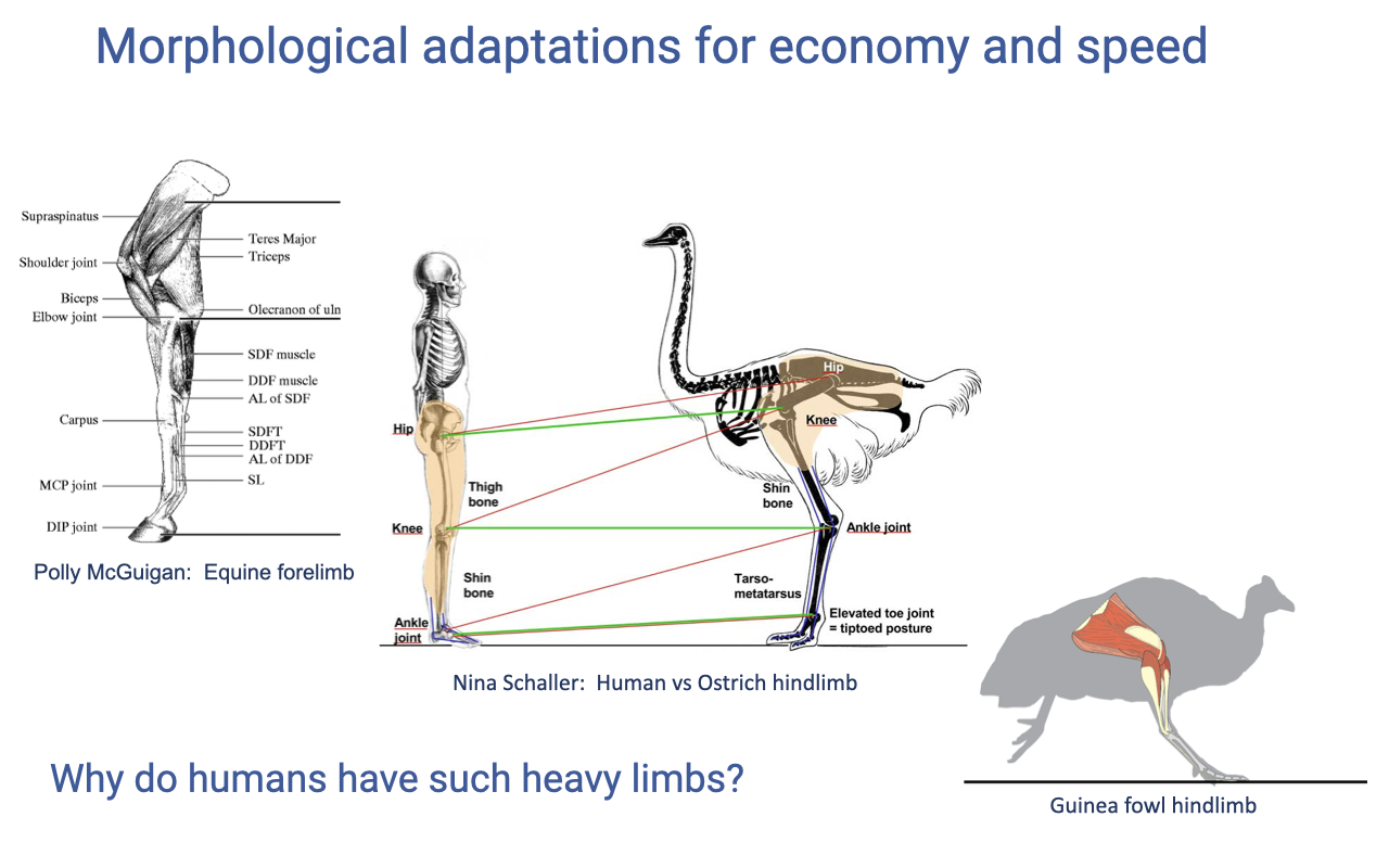
Why Are Human Limbs So Heavy?
- Humans are an outlier among bipedal vertebrates:
- Two legs make up ~half of total body mass — a large fraction relative to specialized cursorial bipeds (ostriches, guinea fowl).
- Compared to ostriches (which have minimal distal-limb mass and very long tendons), humans have substantial distal-limb muscle mass.
- Possible explanations:
- The bird lineage has been bipedal for ~250 million years (back to theropod dinosaurs); humans only ~5 million years — the human bipedal limb may still be a “work in progress.”
- Humans are specialized for a diverse range of tasks (walking, running, climbing, throwing, kicking) — not optimized purely for steady gait.
- Distal-limb mass comes with a metabolic cost (swing energy) but provides versatility.
Slide 29
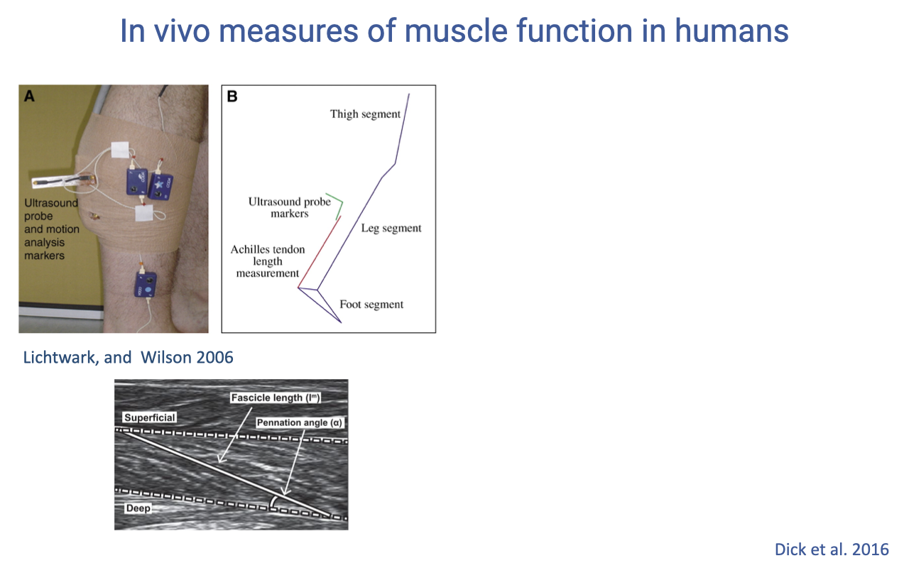
In Vivo Muscle Measurements in Humans — Ultrasound + Motion Capture
- Modern human studies combine:
- B-mode ultrasound taped over the muscle to image fascicle length and pennation angle in real time (Lichtwark & Wilson 2006; Dick et al. 2016).
- Motion capture markers on the ultrasound probe and limb segments to track the Achilles tendon path and MTU length.
- This approach is non-invasive — no implanted instrumentation — and gives essentially the same data as the comparative in vivo experiments in animals.
Slide 30
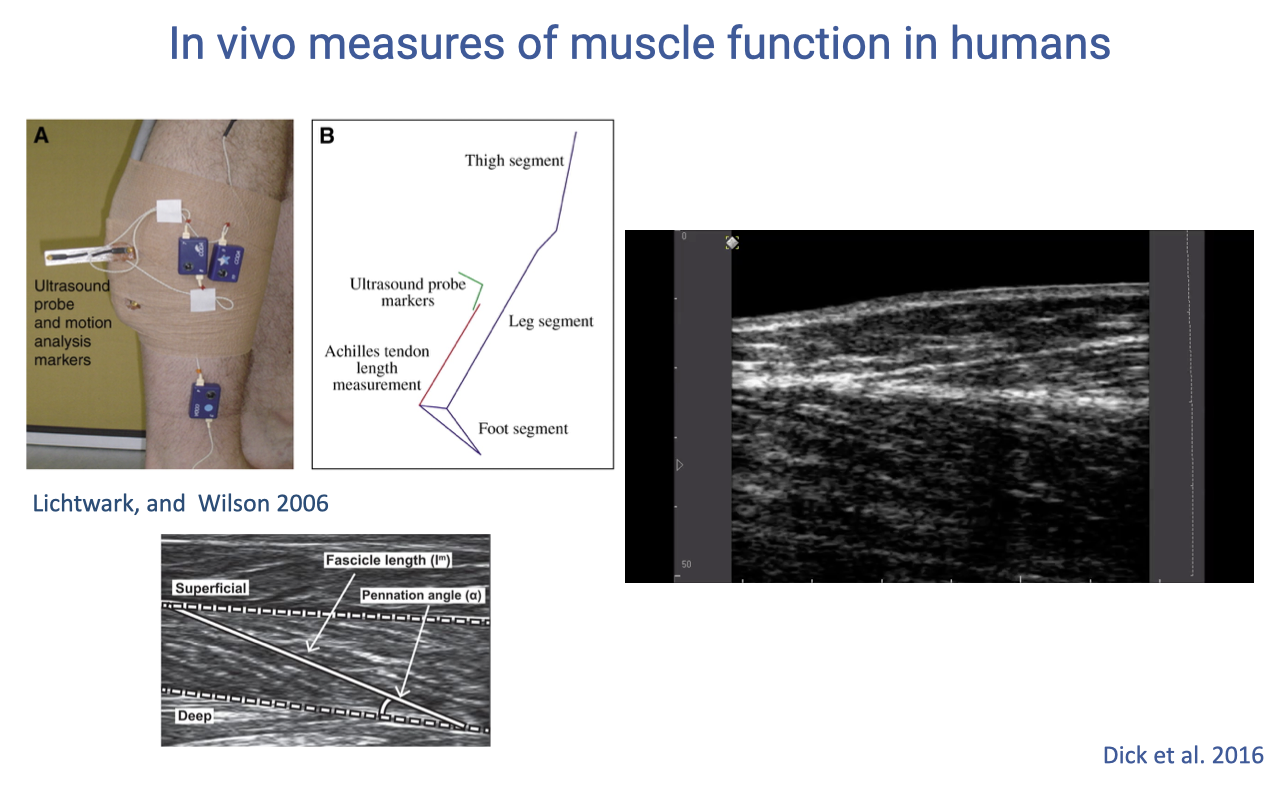
B-Mode Ultrasound — Fascicle Length in Real Time
- Each frame of the B-mode ultrasound video shows the fascicle running between the two aponeuroses at a measurable angle.
- Tracked across many frames, this yields a continuous time-series of fascicle length — the human equivalent of sonomicrometry data from animal experiments.
- Combined with motion capture and force plates, this enables full inverse-dynamics analysis of human walking and running with fascicle-level resolution.
Slide 31
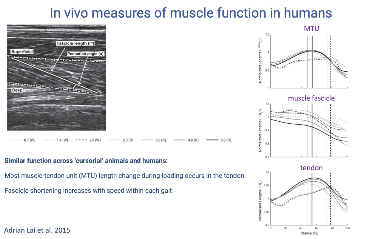
Lai et al. 2015 — Soleus Function in Walking and Running
- Adrian Lai et al. 2015 J Appl Physiol: B-mode ultrasound of human soleus during walking (W) and running (R) at multiple speeds.
- Three coupled length signals over the stance phase:
- MTU length (top): smooth pattern of stretch and recoil.
- Muscle fascicle length (middle): mainly slow shortening — relatively small length change.
- Tendon length (bottom): substantial stretch and recoil.
- Just as in cursorial animals, most of the MTU length change during loading occurs in the tendon. Human soleus operates near-isometrically — strut-like — during gait.
- Fascicle shortening increases with speed within each gait, showing that the soleus modulates its work output as task demands change.
Slide 32
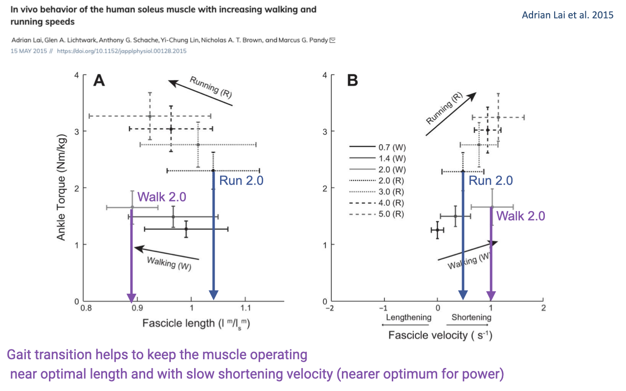
Why People Switch from Walking to Running
- Same speed (e.g., 2.0 m/s), different gait → very different muscle operating conditions:
- Walking 2.0 m/s: fascicle length ~0.9 L0 (suboptimally short for force).
- Running 2.0 m/s: fascicle length ~1.05 L0 (close to optimum) and slower shortening velocity.
- The walk-to-run transition keeps the soleus operating near its optimal F–L and F–V conditions — not just for economy, but for maintaining force capacity as speed increases.
- Connects directly back to the F–L and F–V curves from Lecture 12 — the gait transition is one way humans stay on the optimal portion of the muscle’s intrinsic property surface.
Slide 33
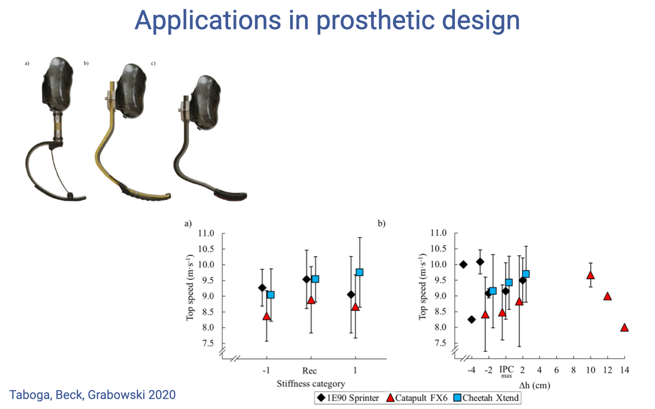
Applications — Running-Blade Prosthetic Design
- The topic — running-blade prosthetics from Taboga, Beck, Grabowski 2020 — directly applies the muscle–tendon spring framework to assistive devices.
- Three prosthetic running blades (1E90 Sprinter, Catapult FX6, Cheetah Xtend) tested in athletes with bilateral lower-limb amputations.
- Stiffness category and height (Δh) of the blade affect top sprint speed — but the optimal value is athlete-specific.
- Designed to mimic the elastic energy cycling behavior of the natural Achilles tendon — but with no muscle to modulate stiffness, blade properties must be tuned to each user.
Slide 34
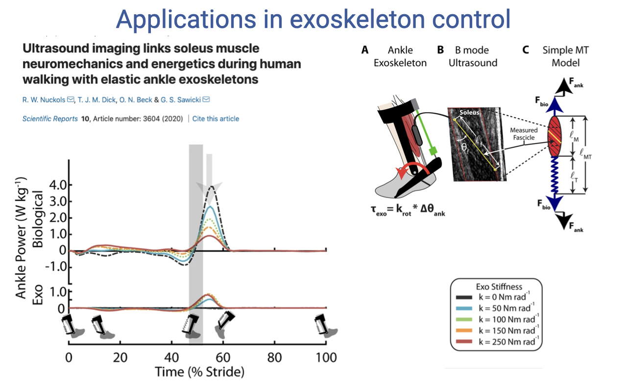
Ankle Exoskeletons and Soleus Function
- Nuckols et al. 2020: passive elastic ankle exoskeletons with stiffness krot that applies torque τexo = krot × Δθank.
- Combined ultrasound (soleus fascicle) + motion capture + indirect calorimetry to measure how the exoskeleton changes biological ankle power during walking.
- As exoskeleton stiffness increases, the biological power (top traces) decreases — the exoskeleton takes over some of the work from the soleus.
- The exoskeleton is essentially an external tendon that adds elastic energy storage in parallel with the Achilles tendon.
Slide 35
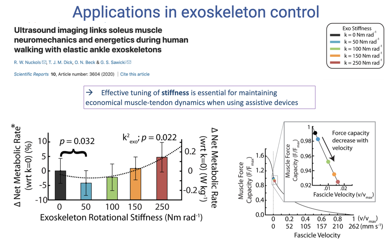
Tuning Exoskeleton Stiffness for Metabolic Benefit
- Energy savings depend on matching exoskeleton stiffness to the wearer’s biological muscle-tendon dynamics:
- Too soft (k = 0): no help from the exoskeleton → no metabolic benefit.
- Just right (k = 50): largest metabolic reduction (~−4% net rate, p = 0.032).
- Too stiff (k = 250): the soleus shortens faster on the F–V curve → reduced force capacity → metabolic cost goes back up.
- Assistive devices interact with the underlying biological muscle F–V relationship. The intrinsic properties from Lecture 12 set the operating envelope that engineers must respect when designing exoskeletons and prosthetics.
- Effective tuning of stiffness is essential for maintaining economical muscle-tendon dynamics with assistive devices.
Slide 36
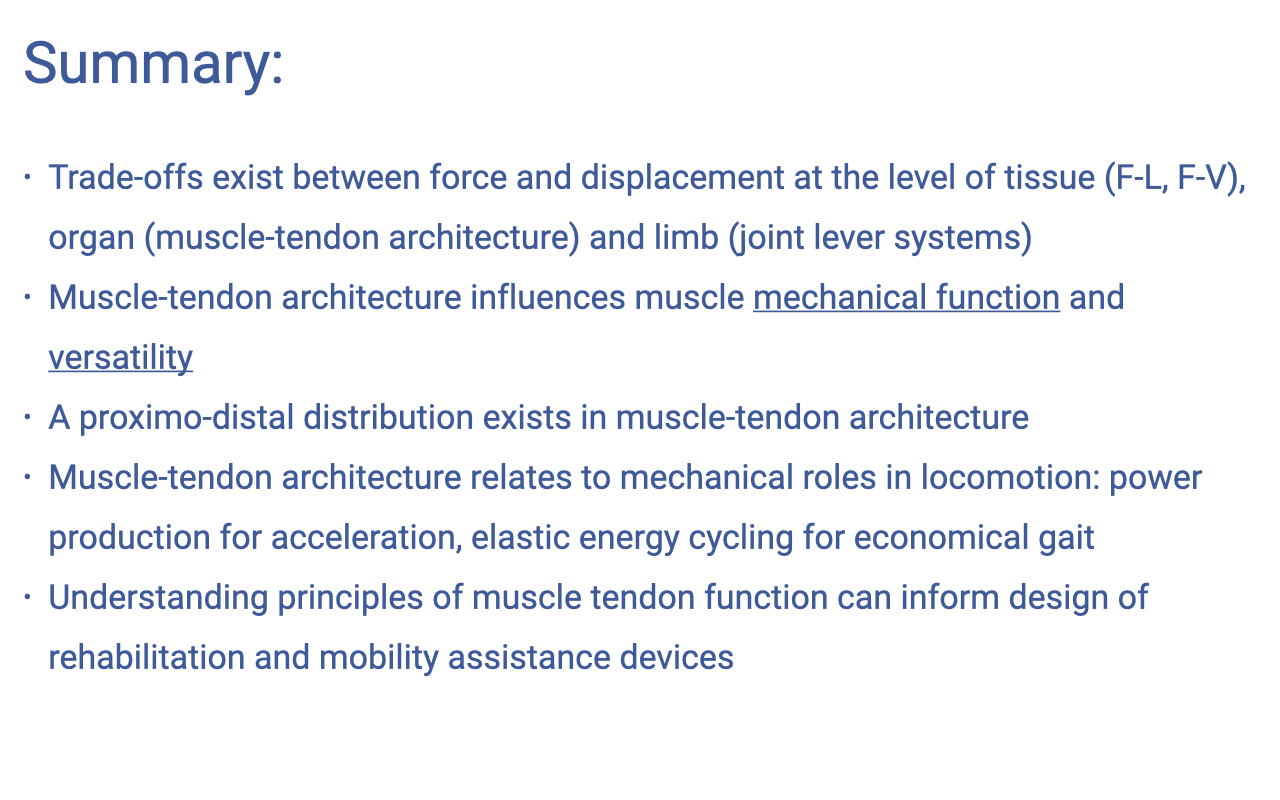
Summary
- Trade-offs between force and displacement appear at every structural level: tissue (F–L, F–V intrinsic properties), organ (muscle–tendon architecture), and limb (joint lever systems).
- Muscle–tendon architecture influences muscle’s mechanical function and versatility — how it can act as motor, spring, or brake depending on task.
- A proximo-distal architectural gradient exists in cursorial limbs: long-fibered, short-tendoned proximal muscles (work and power) vs. short-fibered, long-tendoned distal muscles (elastic cycling, economy).
- These architectural patterns map onto mechanical roles in locomotion: power production for acceleration and incline climbing; elastic energy cycling for economical steady-state gait.
- Understanding muscle–tendon function informs the design of rehabilitation and mobility-assistance devices — prosthetic blades, exoskeletons, surgical interventions.
Slide 37
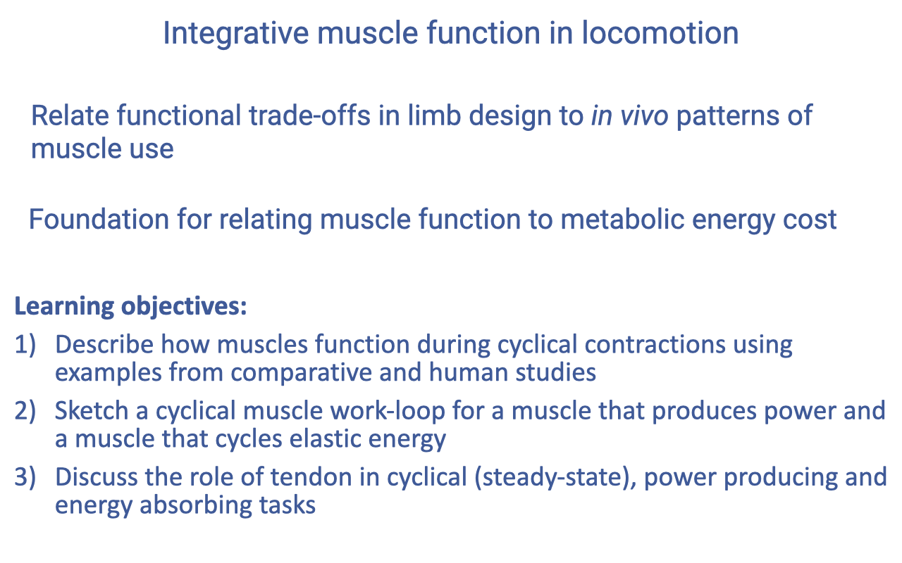
Learning Objectives — Recap
- Cyclical muscle function in real movement is described by work loops — force vs. length plots whose enclosed area is the net work per cycle. In vivo muscle dynamics fall on a continuum from motor to spring.
- A power-producing muscle has a wide, counterclockwise work loop (cockatiel pectoralis, turkey LG on inclines). A spring-like muscle has a tall, narrow loop with most of the MTU length change in the tendon (turkey LG on level, wallaby plantaris, human soleus).
- Tendons act as passive springs that store and return elastic strain energy — minimizing muscle work in steady-state tasks (running, hopping, walking), enabling power amplification in jumping and ballistic tasks, and attenuating power during landings and decelerations.
Key Equations
| Equation | Name | Description |
|---|---|---|
| $F_{muscle} = F_g \times \dfrac{R_g}{r_m}$ | Limb lever equation | Muscle force needed to balance the ground reaction force at a joint, where rm is the muscle moment arm and Rg is the GRF moment arm. |
| $T_h = F_g \times R_h$ | Joint torque (inverse dynamics) | Torque at a joint from the GRF and its moment arm to that joint. |
| $W_h = T_h \times \Delta\theta_{hip}$ | Joint work | Net work at a joint, computed by integrating joint torque through joint angular displacement. |
| $W_{cycle} = \oint F \cdot dL$ | Net work per cycle (work loop) | The line integral of force around a closed length cycle; equal to the area enclosed by the force–length loop. Counterclockwise → positive work; clockwise → negative work. |
| $\tau_{exo} = k_{rot} \times \Delta\theta_{ank}$ | Exoskeleton torque | Passive elastic torque produced by an ankle exoskeleton, with rotational stiffness krot. |
Glossary of Key Terms
| Term | Definition |
|---|---|
| Inverse dynamics | A method for inferring muscle and joint forces from external measurements (motion capture, ground reaction force) by sequentially applying lever-system analysis at each joint. |
| Sonomicrometry | An experimental technique using pairs of small piezoelectric crystals implanted in the muscle; ultrasonic time-of-flight between crystals gives fascicle length during in vivo contraction. |
| Tendon buckle | A surgically implanted strain-gauge transducer that wraps around a tendon and converts tendon deformation into a force signal. |
| B-mode ultrasound | A medical-imaging technique used non-invasively in humans to image muscle fascicle length and pennation angle in real time during movement. |
| Work loop | A force–length plot through one cycle of contraction. Its enclosed area equals the net mechanical work per cycle. Counterclockwise → motor; clockwise → brake; narrow → strut/spring. |
| Motor function | A muscle role in which the muscle actively shortens under load to produce positive net work per cycle — e.g., cockatiel pectoralis in flight, turkey LG on inclines. |
| Spring (strut) function | A muscle role in which the muscle contracts near-isometrically while the tendon stretches and recoils — e.g., wallaby plantaris during hopping, human soleus during running. |
| Brake function | A muscle role in which the muscle generates force while lengthening (eccentric contraction) — absorbing energy. E.g., quadriceps during downhill running. |
| Energy conservation | Energy flow Body → Tendon → Body; the muscle is near-isometric and the tendon cycles elastic energy. Underlies economy of steady-state gait. |
| Power amplification | Energy flow Muscle → Tendon → Body; the muscle slowly stretches the tendon, which then rapidly recoils to release energy at a higher rate than the muscle could produce alone. Underlies jumping and ballistic feeding. |
| Power attenuation | Energy flow Body → Tendon → Muscle; the tendon stretches and the muscle then absorbs the energy eccentrically. Underlies landing and decline running. |
| Proximo-distal gradient | The pattern in cursorial limbs whereby proximal joints are dominated by power-producing muscles and distal joints by spring-like, energy-cycling muscles. |
| Cursorial | Adapted for sustained terrestrial locomotion; many cursorial vertebrates (horses, ostriches, dogs) show extreme proximo-distal architectural gradients. |
| Net joint work | Work done at a joint over a cycle; positive → energy generation; negative → energy absorption; near-zero → spring-like / isometric function. |
| Muscle–tendon unit (MTU) | The functional unit comprising the muscle belly plus its associated tendon (and aponeurosis). |
| Lateral gastrocnemius (LG) | A common ankle extensor used in classic in vivo studies (Roberts 1997 turkey, Daley 2003 guinea fowl). |
| Plantaris | A large ankle extensor in marsupial hoppers; in tammar wallabies it is highly spring-like. |
| Pectoralis | The major downstroke muscle of birds; in cockatiels and many other species, acts purely as a motor with wide counterclockwise work loops. |
| Soleus | A major human ankle extensor; in walking and running it operates near-isometrically (spring-like) with most MTU length change taken up by the Achilles tendon. |
| Achilles tendon | The free distal tendon connecting the triceps surae (gastrocnemius + soleus + plantaris) to the calcaneus; one of the body’s most important elastic-energy storage elements. |
| Walk-to-run transition | The change in human gait that occurs around 2.0 m/s; helps keep muscles like the soleus operating near their optimum F–L and F–V conditions as speed increases. |
| Running blade prosthesis | Carbon-fiber prosthetic limb that mimics the elastic spring behavior of the lower-limb tendons; used by athletes with lower-limb amputations. |
| Ankle exoskeleton | A wearable elastic device that adds parallel rotational stiffness to the ankle joint; reduces metabolic cost when its stiffness is matched to the wearer’s biological muscle–tendon dynamics. |