Lecture 13: Integrative Muscle Structure and Function 3 — Organ and Limb Level
Slide 1

- Opens Lecture 13, the third in the muscle structure-and-function sequence — moving from the cellular (Lecture 11) and tissue (Lecture 12) scales up to the organ (muscle–tendon unit) and limb (skeletal lever) scales.
- Today’s lecture begins with a brief recap of how the intrinsic Hill-type properties of muscle vary with fiber type, activation, and operating velocity, and how those tissue-level properties shape whole-body performance.
- It then introduces the next layer of structure: muscle–tendon architecture (PCSA, fascicle length, pennation, tendon design) and skeletal lever systems (moment arms, torque balance, effective mechanical advantage).
Slide 2
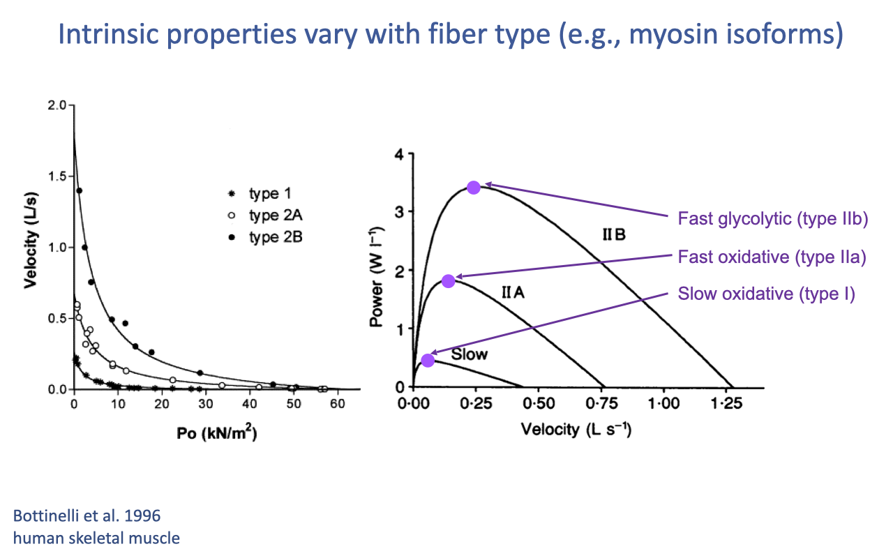
Recap — Hill-Type Properties Vary With Fiber Type
- The intrinsic Hill-type properties (force–length, force–velocity, and power–velocity) define the maximum performance envelopes of muscle — and these envelopes shift systematically with fiber type.
- Fiber-type variation is driven primarily by which myosin heavy chain isoform the fiber expresses, with parallel variation in other contractile proteins (troponin, tropomyosin, SERCA isoforms).
- In human skeletal muscle (Bottinelli et al. 1996):
- Type IIB (fast glycolytic): highest Vmax and highest peak power, at the highest optimum velocity.
- Type IIA (fast oxidative): intermediate.
- Type I (slow oxidative): lowest Vmax, lowest peak power, at the slowest optimum velocity.
- All three curves share the same fundamental hyperbolic shape — only their scale and curvature differ. This is why fiber-type composition of a muscle is so important for sport-specific performance.
Slide 3
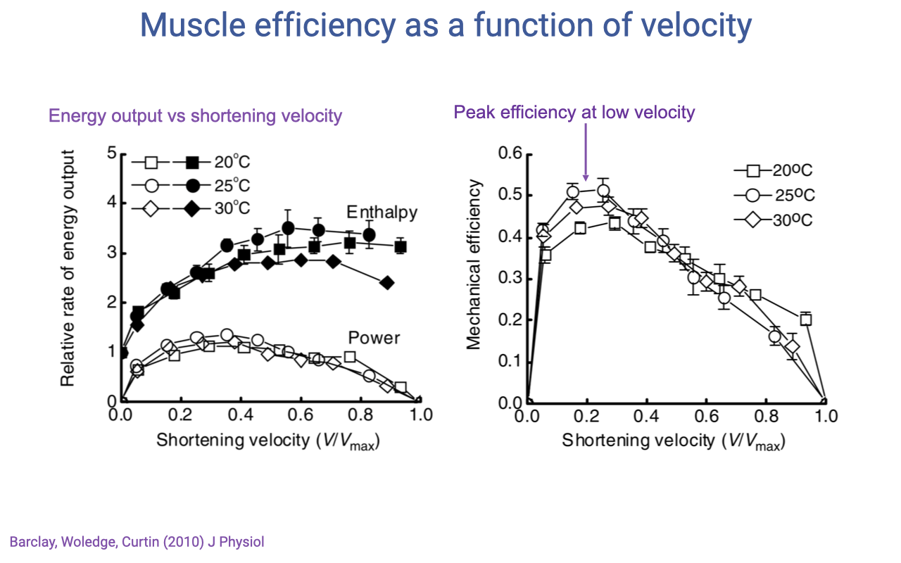
Recap — Muscle Efficiency Peaks at Low Velocity
- Mechanical efficiency = mechanical work output ÷ total energy expenditure (work + heat).
- Across temperatures (20–30°C in mouse soleus), efficiency:
- Peaks at low shortening velocity (~0.1–0.2 V/Vmax).
- Falls off at higher velocities as more energy is lost as heat during rapid cross-bridge cycling.
- The velocity that maximizes power (~0.2–0.3 V/Vmax) is higher than the velocity that maximizes efficiency (~0.1–0.2 V/Vmax).
- Animals (and athletes) face a fundamental trade-off between going fast (peak power) and using fuel economically (peak efficiency). The optimal contraction velocity depends on which currency the task is optimizing.
Slide 4
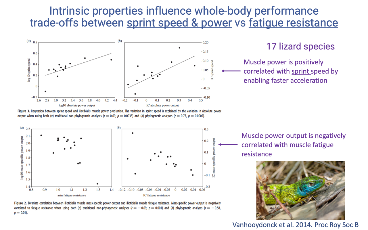
Tissue Properties Predict Whole-Body Performance — Lizards
- Tissue-level intrinsic properties can directly predict whole-body locomotor performance — and the same trade-offs visible at the cellular level reappear at the organismal level.
- Across 17 lizard species (Vanhooydonck et al. 2014):
- Mass-specific muscle power is positively correlated with sprint speed — high-power muscle enables faster acceleration.
- Mass-specific muscle power is negatively correlated with fatigue resistance — species with high power have less endurance.
- This is the whole-organism manifestation of the cellular zero-sum game from Lecture 11 and the F–V trade-off from Lecture 12: each species sits at a different point on the same trade-off surface, set by its ecological niche.
Slide 5
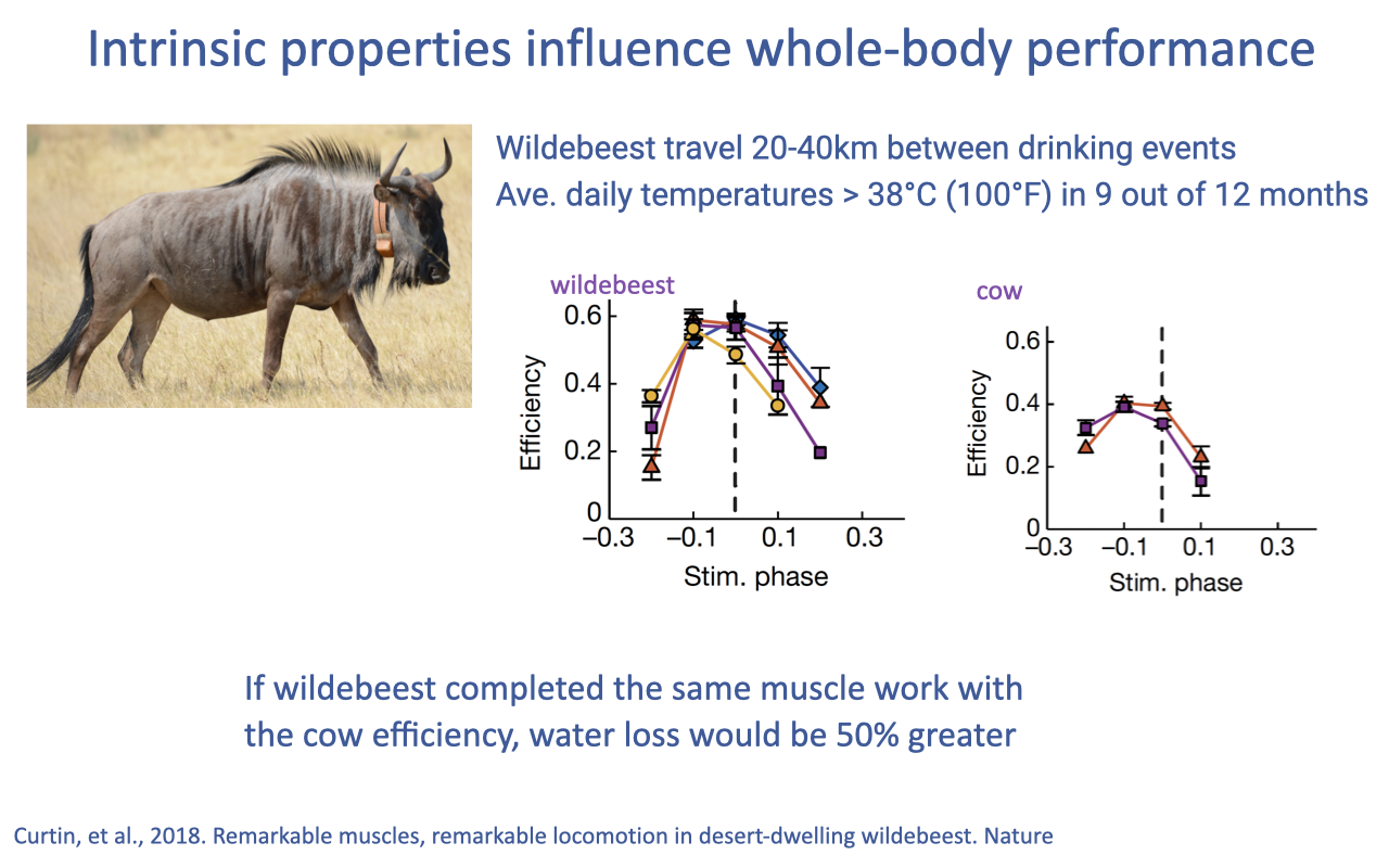
Tissue Properties Predict Whole-Body Performance — Wildebeest Efficiency
- A second example linking tissue-level efficiency to whole-body performance: the migrating wildebeest.
- Wildebeest travel 20–40 km between drinking events in temperatures above 38°C (100°F) for 9 of 12 months — a punishing combination of locomotor and thermal demand.
- Curtin et al. (2018) Nature: wildebeest red muscle achieves peak efficiency ~0.6 (60%) — roughly 50% higher than typical mammalian muscle (cow: ~0.4).
- Why the very high efficiency matters: low-efficiency muscle generates more heat for the same mechanical work, and dissipating that heat costs water (sweat, panting). The authors estimate that if wildebeest used cow-like muscle efficiency, water loss during migration would be ~50% greater.
- This is a clean example of how selection on muscle’s intrinsic properties can be driven by the integrated thermal and water-balance demands of an animal’s ecology.
Slide 6
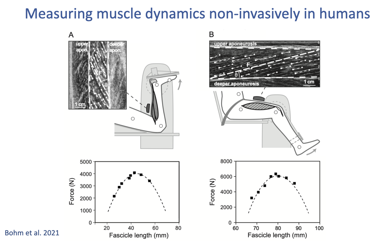
Measuring Intrinsic Properties Non-Invasively in Humans
- For decades, the F–L and F–V curves in Lectures 12–13 came from isolated-muscle bench-top experiments (mostly on animals). Modern techniques now allow these curves to be measured non-invasively in humans.
- Two methods are combined (Bohm et al. 2021):
- Dynamometer: a rigid rig that fixes joint angle and measures the resulting joint torque while the subject contracts maximally — the human equivalent of the muscle ergometer.
- B-mode ultrasound: a probe taped over the muscle images fascicle length and pennation angle in real time during the contraction.
- Combining the two yields a direct fascicle-level F–L curve for individual human muscles. Different muscles (panel A vs. panel B) show different optimum lengths and force ranges.
- This opens the door to measuring subject-specific intrinsic properties — important for sport science, rehabilitation, and personalized musculoskeletal modeling.
Slide 7
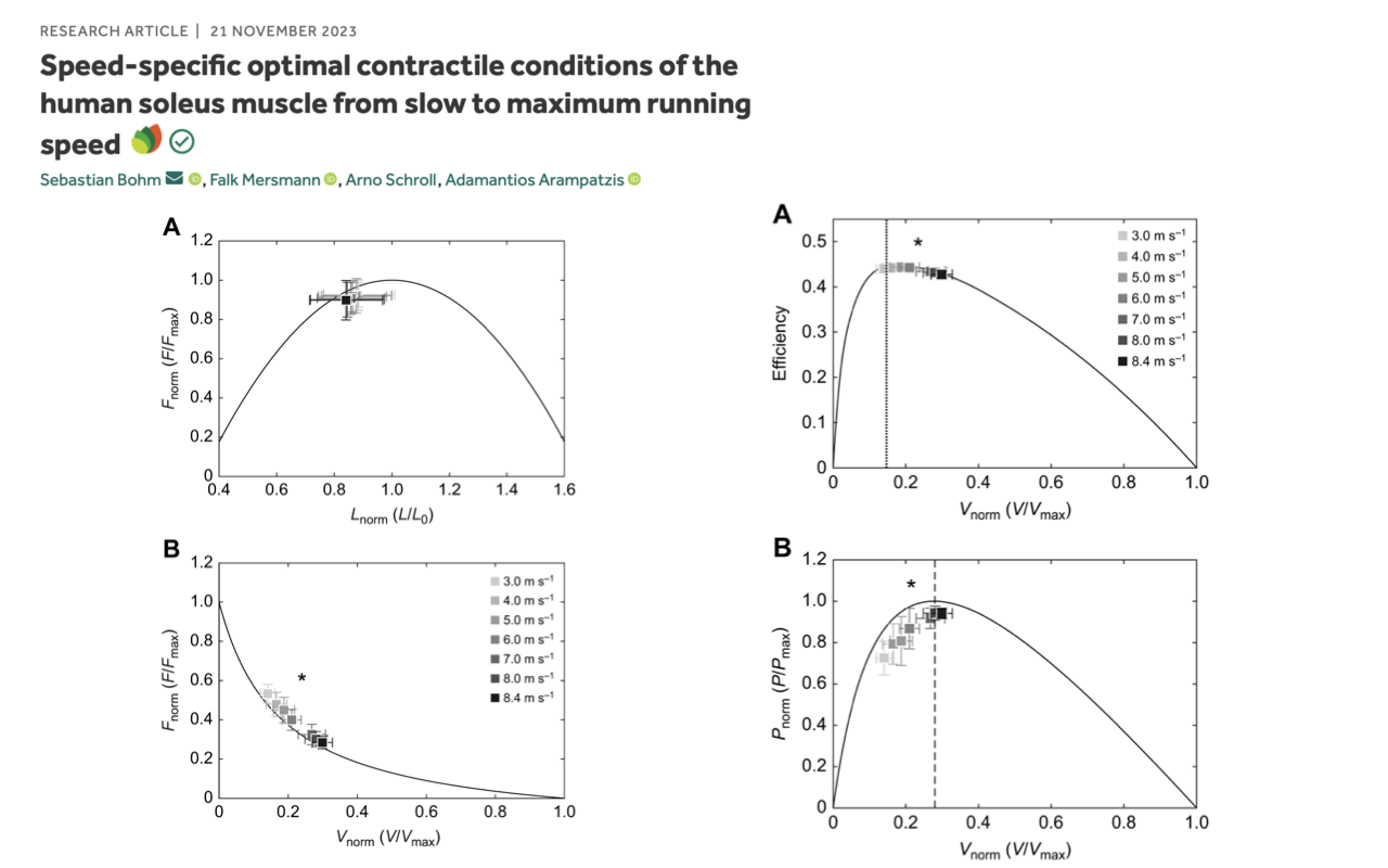
Operating Range Shifts From Economy to Power With Speed
- Bohm et al. 2023 combined dynamometer and ultrasound to measure how the human soleus operates on its own F–L–V envelope during running at speeds from 3.0 to 8.4 m/s.
- Each set of points shows the soleus’s operating point at one running speed, plotted on the muscle’s own intrinsic curves:
- Top-left (F–L plane): at all speeds, the soleus operates near L/L0 ≈ 0.8–1.0 — close to the plateau for maximum force.
- Top-right (Efficiency–V): at slower running speeds, the soleus operates near V/Vmax ≈ 0.2 — the peak efficiency region.
- Bottom plots (F–V and P–V): as running speed increases, the operating point shifts rightward along the F–V curve toward higher velocities, and along the power curve toward the optimum velocity for peak power (~0.3 V/Vmax).
- The soleus is not stuck at one operating condition. As running speed increases, it shifts from the economy regime (low velocity, near-isometric) toward the power regime (intermediate velocity, near-peak power) — a real-time demonstration of the trade-offs visualized on the F–V curve.
Slide 8
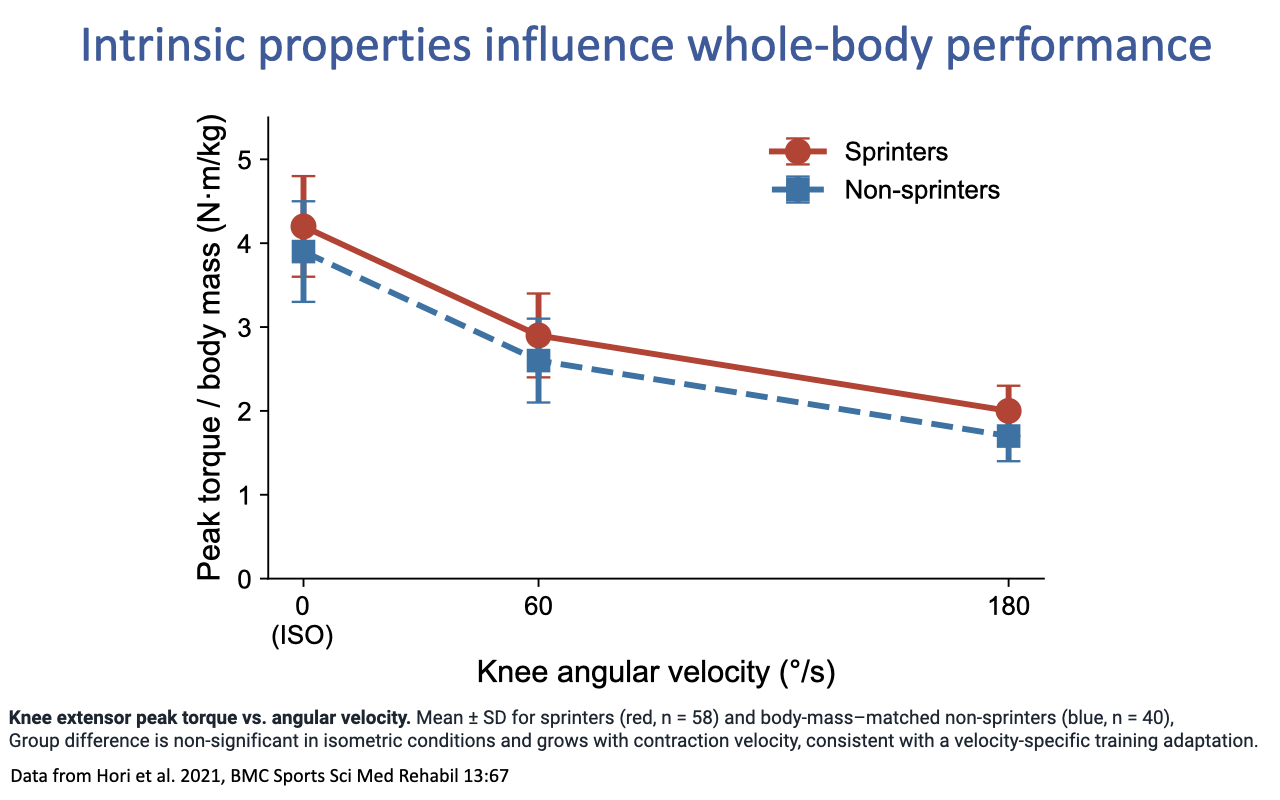
Sprinters vs. Non-Sprinters — Velocity-Specific F–V Adaptation
- A direct human comparison of intrinsic properties between elite sprinters (n = 58) and body-mass-matched non-sprinters (n = 40) (Hori et al. 2021):
- At isometric conditions (0°/s), the two groups produce similar peak knee-extensor torque — maximum static strength is not the differentiator.
- As contraction velocity rises (60°/s, 180°/s), sprinters maintain higher torque than non-sprinters — a velocity-specific advantage that grows with speed.
- Interpretation: the difference between sprinters and non-sprinters is not raw force but the shape of the F–V curve — sprinters resist the velocity-dependent decline in force more effectively, consistent with a velocity-specific training adaptation (and/or a fast-fiber-type genetic predisposition).
- This neatly closes the loop from cellular fiber type (Slide 2) → tissue-level F–V curve (Lecture 12) → comparative animal performance (Slides 4–5) → individual human performance differences.
Slide 9
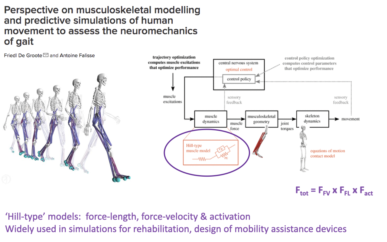
Why Hill-Type Properties Matter — Musculoskeletal Modeling
- The intrinsic F–L and F–V properties are the foundation of musculoskeletal models used in clinical and research biomechanics.
- A predictive simulation of human walking can be built from a subject’s motion-capture video alone, run through a forward model with Hill-type muscle elements:
- These models are used for rehabilitation planning, prosthetic and orthotic design, surgical planning (e.g., tendon transfers), and the design of mobility-assistance devices (exoskeletons).
- Hill-type models capture F–L, F–V, and activation effects but do not capture all of the complexities of contraction (e.g., shape changes with activation level, history-dependent effects, muscle-tendon interaction). The next slide highlights one of those limitations directly.
Slide 10
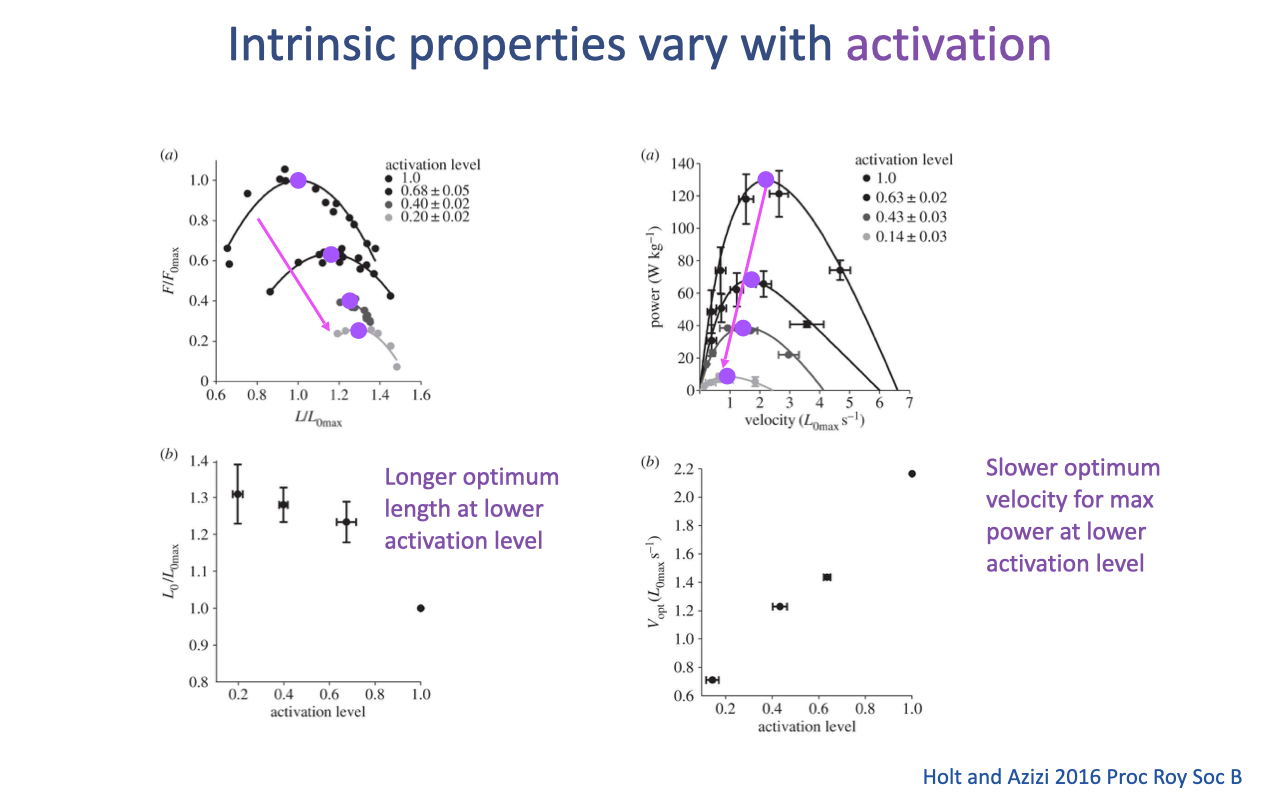
Recap — Intrinsic Properties Vary With Activation
- Hill-type properties are not fixed — they depend on activation level (Holt and Azizi 2016).
- At lower activation levels (more typical of natural submaximal movements):
- F–L curve shifts to the right → optimum length L0 shifts to longer fiber lengths.
- Power–V curve shifts left and down → optimum velocity for peak power Vopt shifts to slower velocities.
- This is a known limitation of standard Hill-type models (Slide 9), which assume activation only multiplicatively scales the curve. Building better models that capture activation-dependent shape changes is an active area of research — and important for predicting muscle function in real, dynamic tasks.
Slide 11
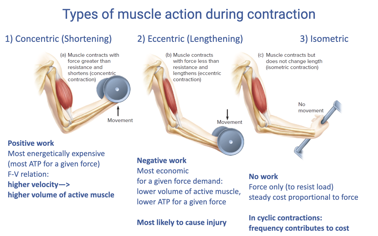
Types of Muscle Action — Concentric, Eccentric, Isometric
| Action | Description | Work | Energetic cost |
|---|---|---|---|
| Concentric (shortening) | Fmuscle > load; muscle shortens | Positive | Most expensive ATP per unit force; via the F–V relation, higher velocity demands a higher volume of active muscle |
| Eccentric (lengthening) | Fmuscle < load; muscle lengthens | Negative | Most economic — for a given force demand, lower volume of active muscle and lower ATP per unit force; highest injury risk |
| Isometric | No length change; force only, to resist load | None | Steady-state cost proportional to force; in cyclic contractions, frequency itself contributes to cost |
- These distinctions are foundational for the rest of the lecture: a single muscle will perform very different work depending on whether it acts concentrically, eccentrically, or isometrically during a given task.
- The relevance to architecture (next slides): a muscle’s fiber length, pennation, and tendon design strongly influence how much active fiber volume is required to do the same external task — and therefore how much ATP it costs.
Slide 12
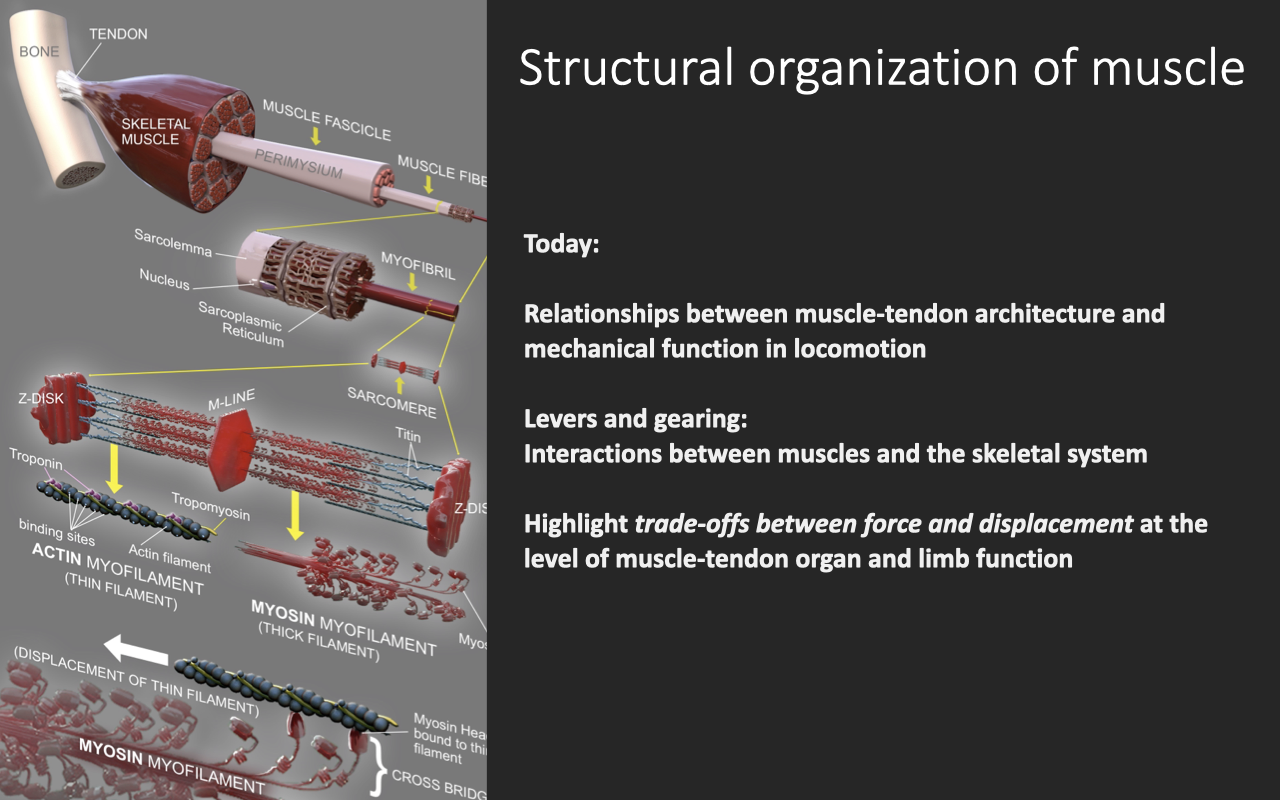
Today — From Tissue to Organ to Limb
- The recap is over — today’s new content builds upward in scale from the tissue-level properties:
- Organ-level: muscle–tendon architecture (fascicle length, pennation angle, PCSA, tendon length and stiffness) and how it sets force, displacement, velocity, work, and power capacity at the whole muscle–tendon unit (MTU) level.
- Limb-level: the lever and gearing systems through which muscles act on bones and joints.
- Central theme: a trade-off between force and displacement appears at each level — independent of, but compounding with, the tissue-level trade-offs.
Slide 13
Learning Objectives
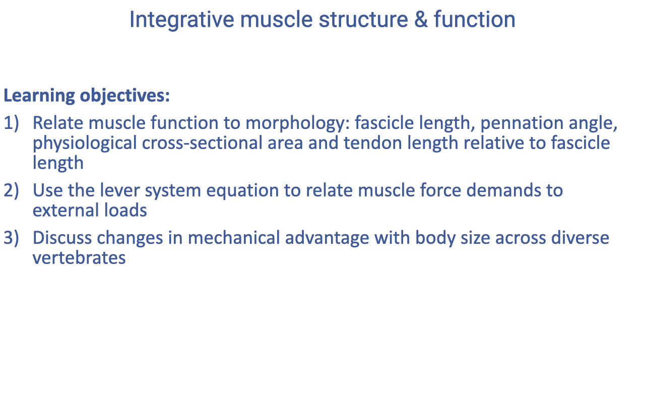
- Relate muscle function to morphology: fascicle length, pennation angle, physiological cross-sectional area (PCSA), and tendon length relative to fascicle length.
- Use the lever-system equation to relate muscle-force demands to externally applied loads at a joint.
- Discuss how effective mechanical advantage (EMA) scales with body size across diverse vertebrates.
Slide 14
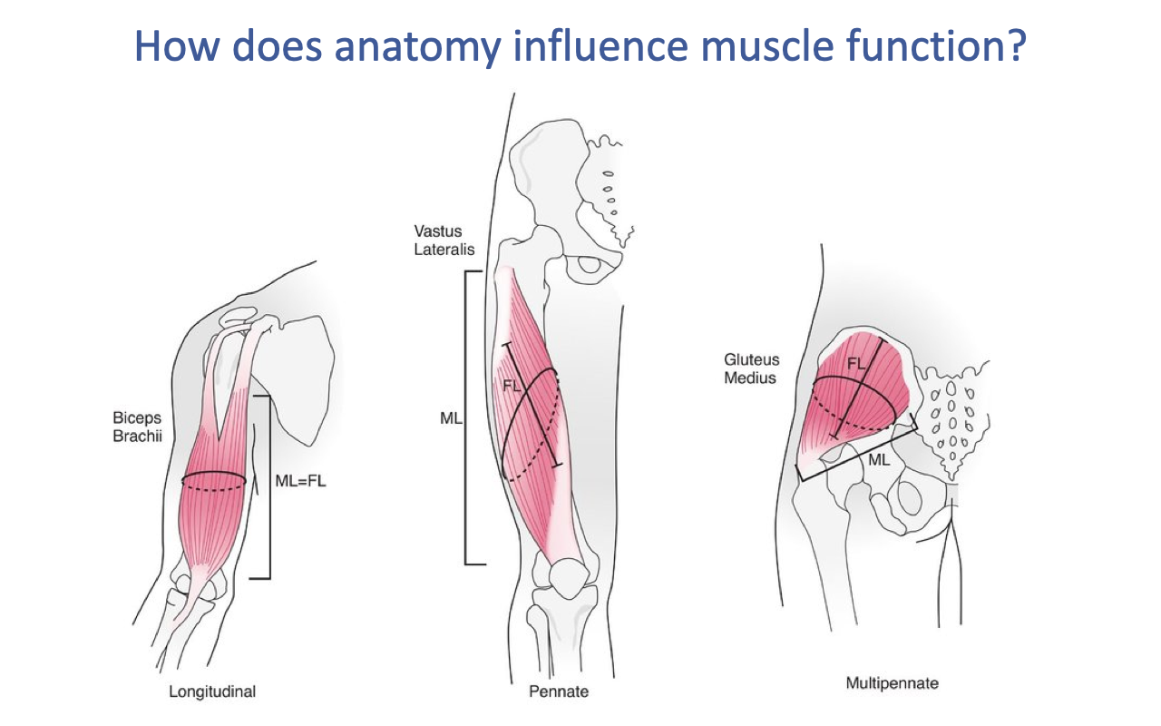
Three Architectural Categories
- Skeletal muscles fall on a continuum of architectural designs, illustrated by three textbook examples:
- Longitudinal (parallel-fibered) — e.g., biceps brachii: fibers run along the line of action; muscle length ≈ fascicle length (ML = FL).
- Unipennate / pennate — e.g., vastus lateralis: fibers act at an angle (the pennation angle) to the line of action; muscle length > fascicle length.
- Multipennate — e.g., gluteus medius: multiple internal tendons with fibers fanning at multiple angles; cannot be characterized by a single pennation angle.
- These categories influence the muscle’s force, displacement, velocity, work, and power capacities for a given volume of muscle.
Slide 15
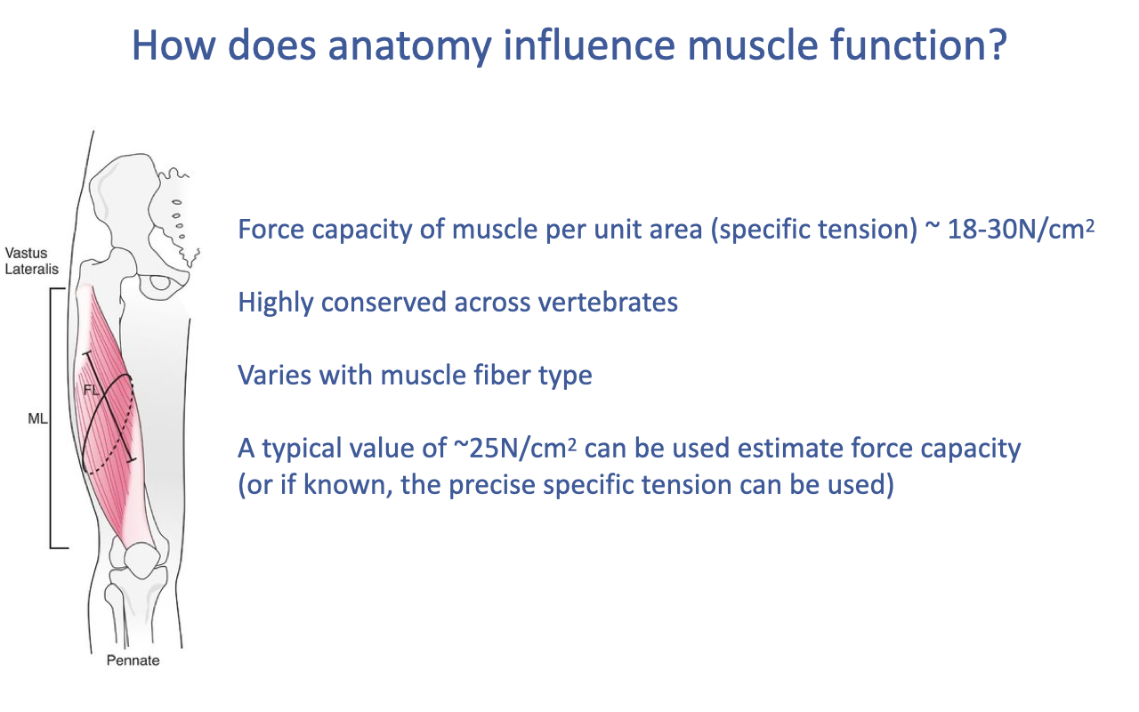
Specific Tension — A Conserved Tissue Property
- Specific tension (force per unit cross-sectional area of contractile tissue) is highly conserved across vertebrates:
- The range reflects fiber-type variation:
- Anaerobic fast-twitch fibers (high myofibril fraction) → higher specific tension.
- Aerobic / slow-twitch fibers → lower specific tension.
- This conservation lets researchers scale forces between species and estimate whole-muscle force from anatomical measurements.
- A typical value of ~25 N/cm² is used as an estimate when the precise specific tension is not known.
Slide 16
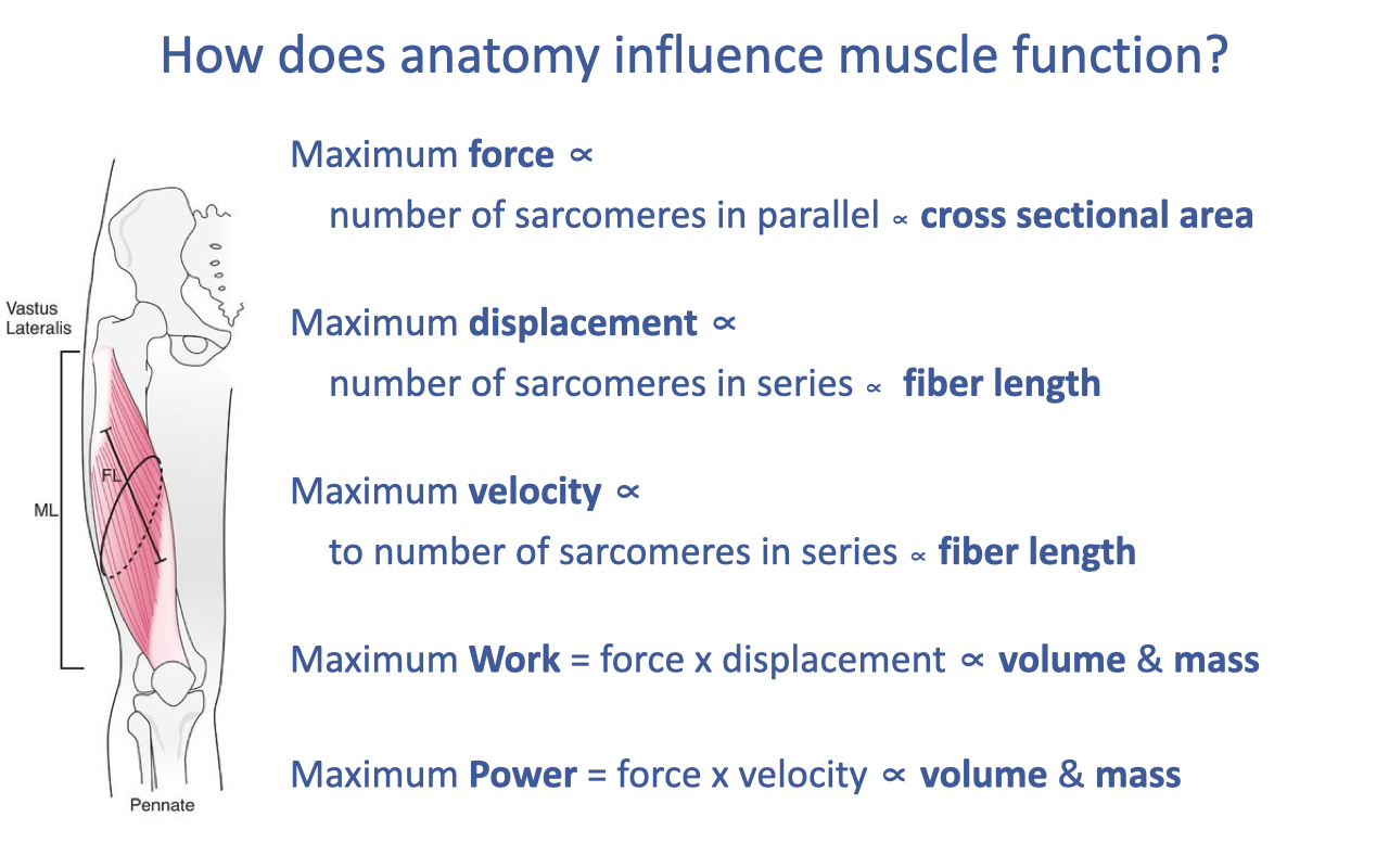
Architectural Relationships — Force, Displacement, Velocity, Work, Power
- Maximum force ∝ number of sarcomeres in parallel ∝ cross-sectional area.
- Maximum displacement ∝ number of sarcomeres in series ∝ fiber length.
- Maximum velocity ∝ number of sarcomeres in series ∝ fiber length.
- Maximum work = force × displacement ∝ volume ∝ mass.
- Maximum power = force × velocity ∝ volume ∝ mass.
- A clean way to remember the architecture rules: the muscle’s cross-sectional area sets force; its fiber length sets displacement and velocity; its volume (and therefore mass) sets work and power.
- This is also why muscle mass is so often used as a proxy for power capacity in comparative studies — muscle has a highly conserved density (~1.06 g/cm³), so mass and volume are tightly coupled.
Slide 17
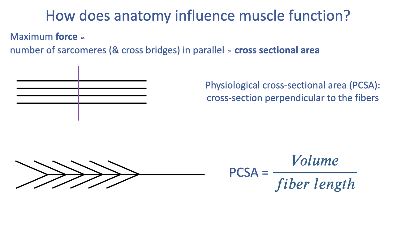
Physiological Cross-Sectional Area (PCSA)
- For a parallel-fibered muscle, PCSA is just a transverse cut perpendicular to the fibers.
- For a pennate or multipennate muscle, the fibers cross the muscle belly at angles — a single transverse cut does not give the correct cross-section.
- The general formula avoids the geometry problem entirely:
- Volume can be measured by:
- Mass × density in dissection (muscle density is highly conserved at ~1.06 g/cm³).
- Imaging (MRI, CT, ultrasound) in living human studies.
- Fiber length is measured as the average length of dissected fascicles (or estimated from imaging).
Slide 18
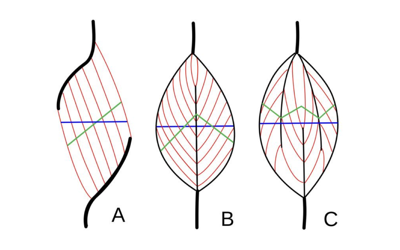
Anatomical vs. Physiological Cross-Sections
- The blue lines show a transverse section through the muscle belly perpendicular to the long axis of the muscle — what an anatomist might cut in dissection.
- The green lines show the actual physiological cross-section perpendicular to the fiber axis — the cross-section that the active sarcomeres present.
- For complex muscles like the soleus (which internally resembles option C — many compartments with short fibers on internal tendons), there is no simple cut that yields the PCSA.
- In these cases, only the Volume / fiber length formula is practical.
Slide 19
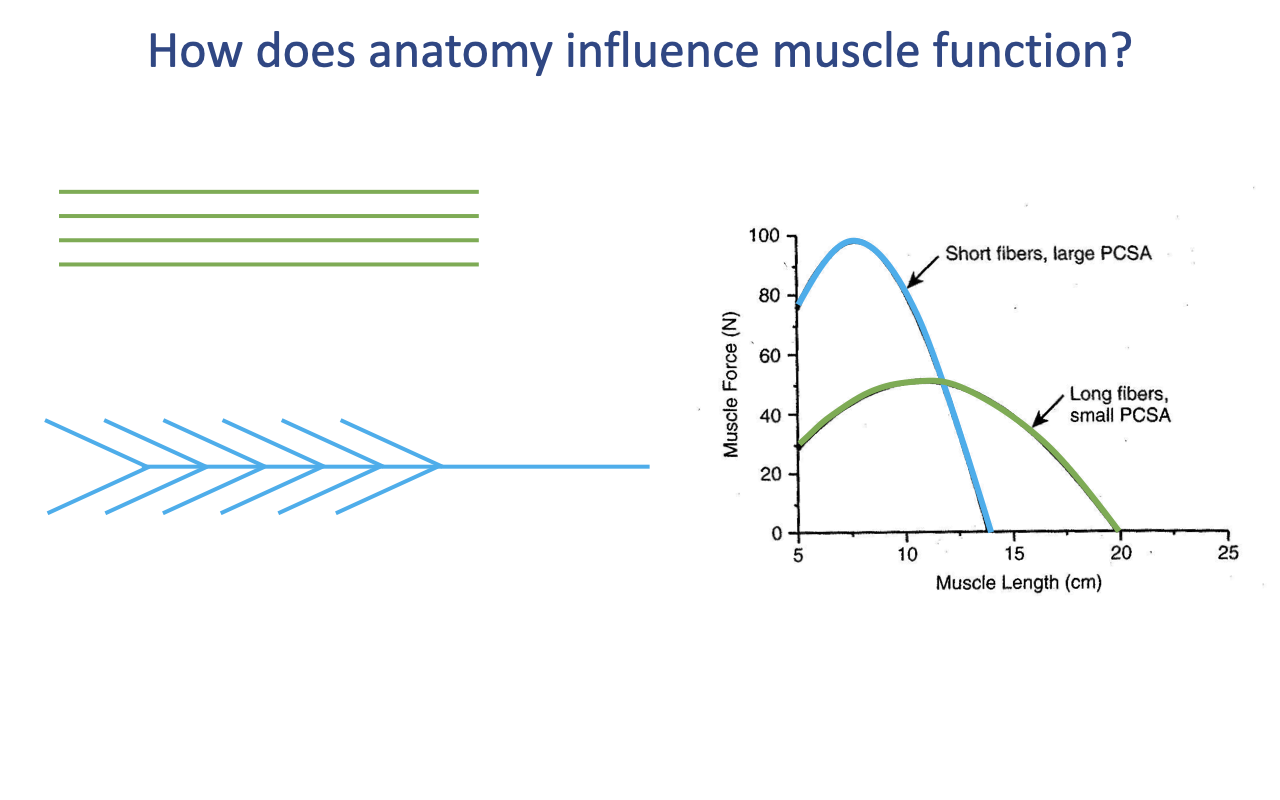
Architectural Force–Length Trade-off
- Two hypothetical muscles with the same volume but different architectures:
- Short fibers, large PCSA (e.g., a bipennate calf-like muscle) → high peak force but a narrow operating range.
- Long fibers, small PCSA (e.g., a parallel-fibered biceps-like muscle) → lower peak force but a wider operating range.
- This is a whole muscle–tendon unit (MTU) level force–length trade-off that adds to the tissue-level force–length curve.
- High-PCSA muscles are best for brief high-force tasks within a narrow range; long-fibered muscles are best for large excursions at moderate force.
Slide 20
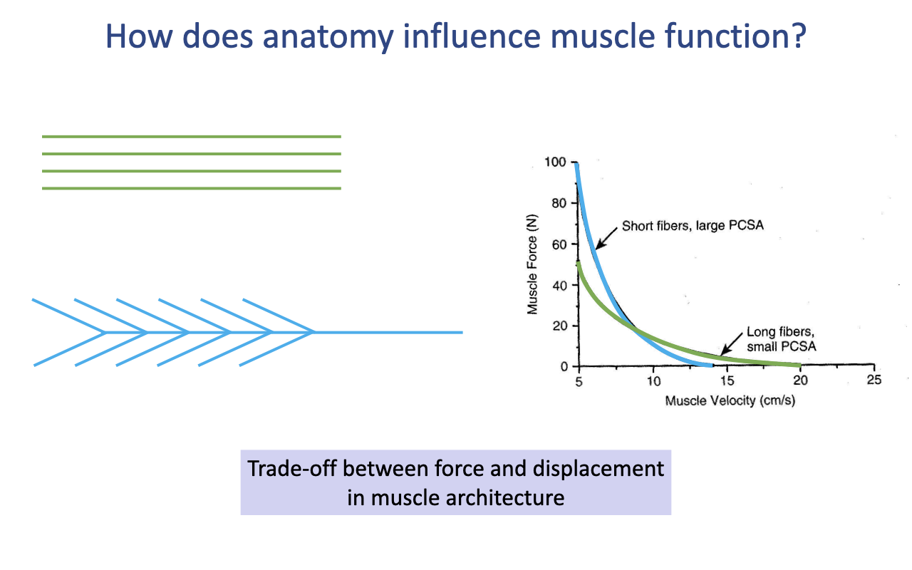
Architectural Force–Velocity Trade-off
- The same architectural trade-off appears in the F–V relationship at the MTU level:
- Short fibers, large PCSA → higher Fmax but lower Vmax (steeper drop with velocity).
- Long fibers, small PCSA → lower Fmax but higher Vmax (more gradual drop).
- This trade-off is independent of fiber type — it arises purely from muscle architecture and applies even when both muscles have identical tissue-level intrinsic properties.
- The whole-muscle F–V curve combines fiber-type effects (Slide 2) with architectural effects (this slide) into a single envelope.
Slide 21
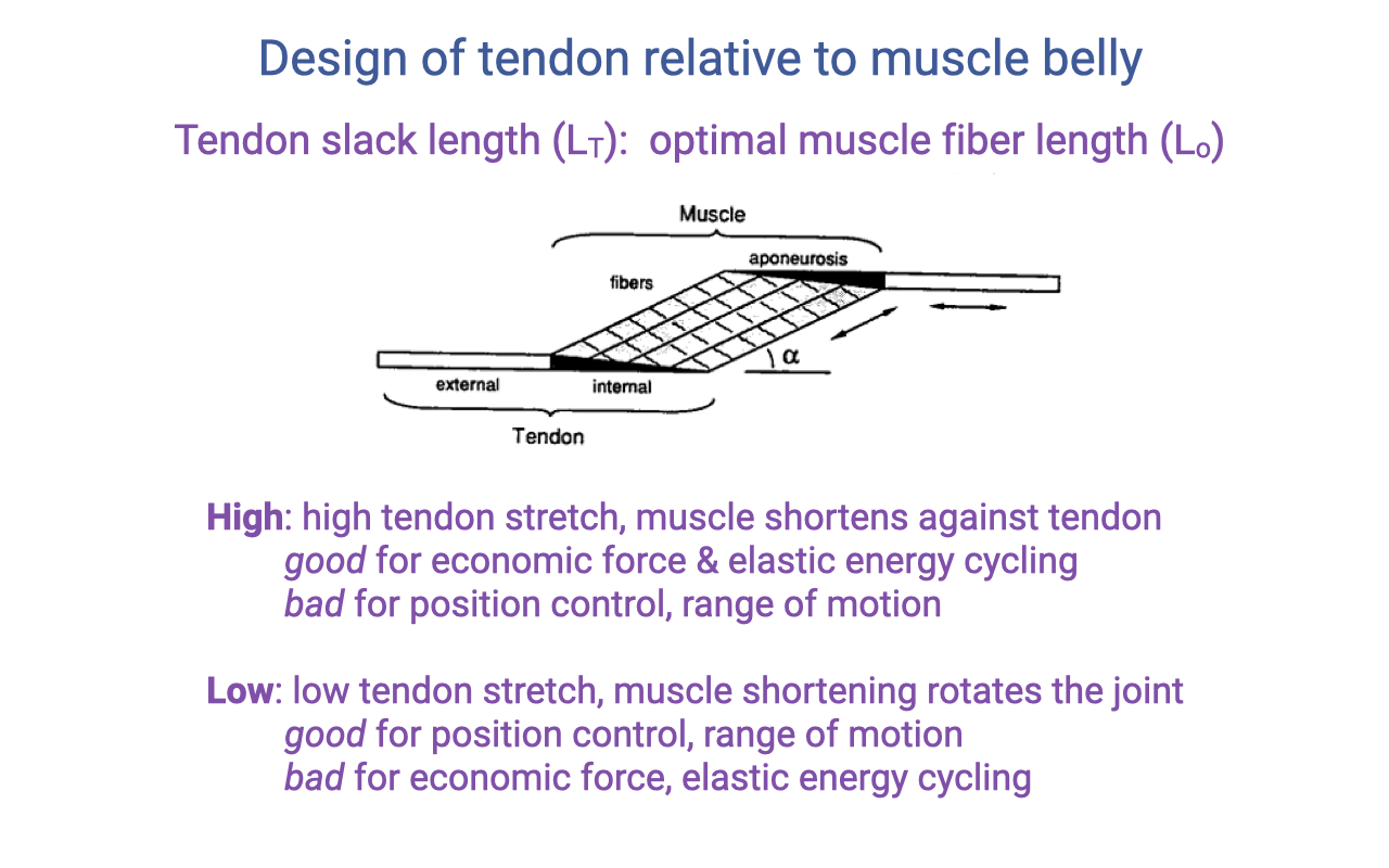
Tendon Slack Length to Optimal Fiber Length Ratio (LT / Lo)
- A second architectural parameter: the ratio of tendon slack length (LT, including both aponeurosis and external tendon) to optimal muscle fiber length (Lo).
- High LT/Lo ratio (long tendon, short fibers):
- The tendon stretches a lot under load → muscle effectively shortens against the tendon.
- Good for economic force and elastic energy cycling.
- Bad for joint position control and range of motion.
- Low LT/Lo ratio (short tendon, long fibers):
- Muscle shortening directly rotates the joint.
- Good for position control and range of motion.
- Bad for elastic energy storage and economic force.
Slide 22
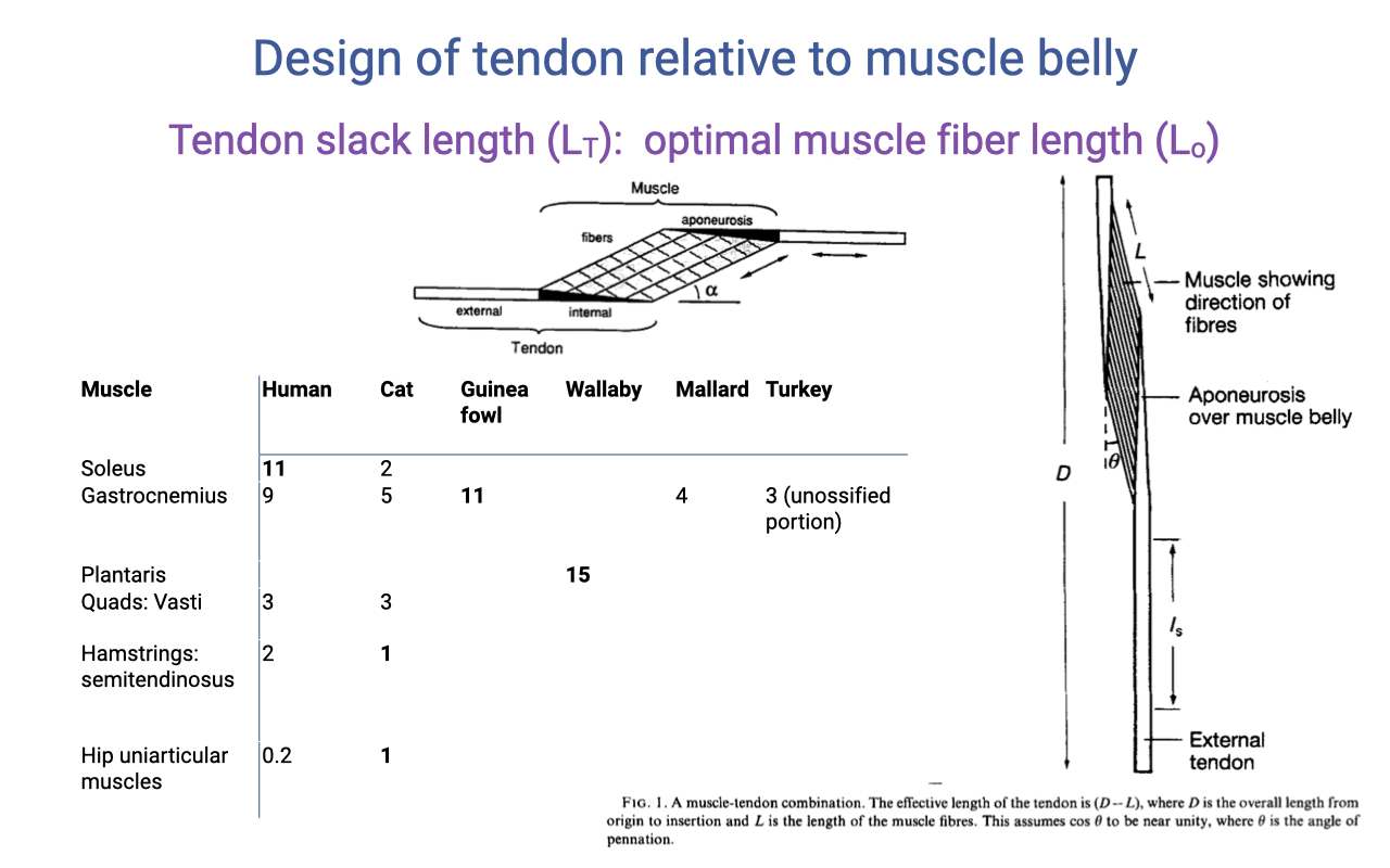
Comparative LT/Lo Ratios — Distal vs. Proximal
| Muscle | Human | Cat | Guinea fowl | Wallaby | Mallard | Turkey |
|---|---|---|---|---|---|---|
| Soleus | 11 | 2 | — | — | — | — |
| Gastrocnemius | 9 | 5 | 11 | — | 4 | 3 |
| Plantaris | — | — | — | 15 | — | — |
| Quads (vasti) | 3 | 3 | — | — | — | — |
| Hamstrings (semitendinosus) | 2 | 1 | — | — | — | — |
| Hip uniarticular muscles | 0.2 | 1 | — | — | — | — |
- A clear pattern: distal limb muscles (soleus, gastrocnemius, plantaris) have very high LT/Lo ratios (~5–15) — long tendons relative to short fibers, optimized for elastic energy cycling.
- Proximal hip muscles have low ratios (~0.2–3) — short tendons, longer fibers, optimized for range of motion, work, and power.
- Muscles typically only shorten by ~25% of their length in a single contraction. Combined with high LT/Lo, this means most of the MTU length change comes from tendon stretch, not fiber shortening.
Slide 23
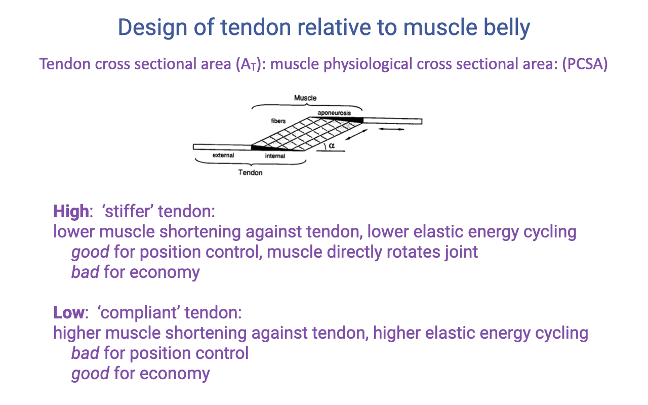
Tendon Cross-Sectional Area to PCSA Ratio (AT / PCSA)
- A third architectural parameter: the ratio of tendon cross-sectional area to muscle PCSA. This sets how stiff the tendon is relative to the force the muscle can generate.
- High AT/PCSA → stiff tendon:
- Lower muscle shortening against the tendon, lower elastic energy cycling at a given force.
- Good for position control — the muscle directly rotates the joint.
- Bad for economy.
- Low AT/PCSA → compliant tendon:
- Higher muscle shortening against the tendon, higher elastic energy cycling at a given force.
- Bad for position control.
- Good for economy.
- Combined with the LT/Lo ratio (Slide 21), AT/PCSA defines whether the MTU behaves as a spring or a direct-drive actuator.
Slide 24
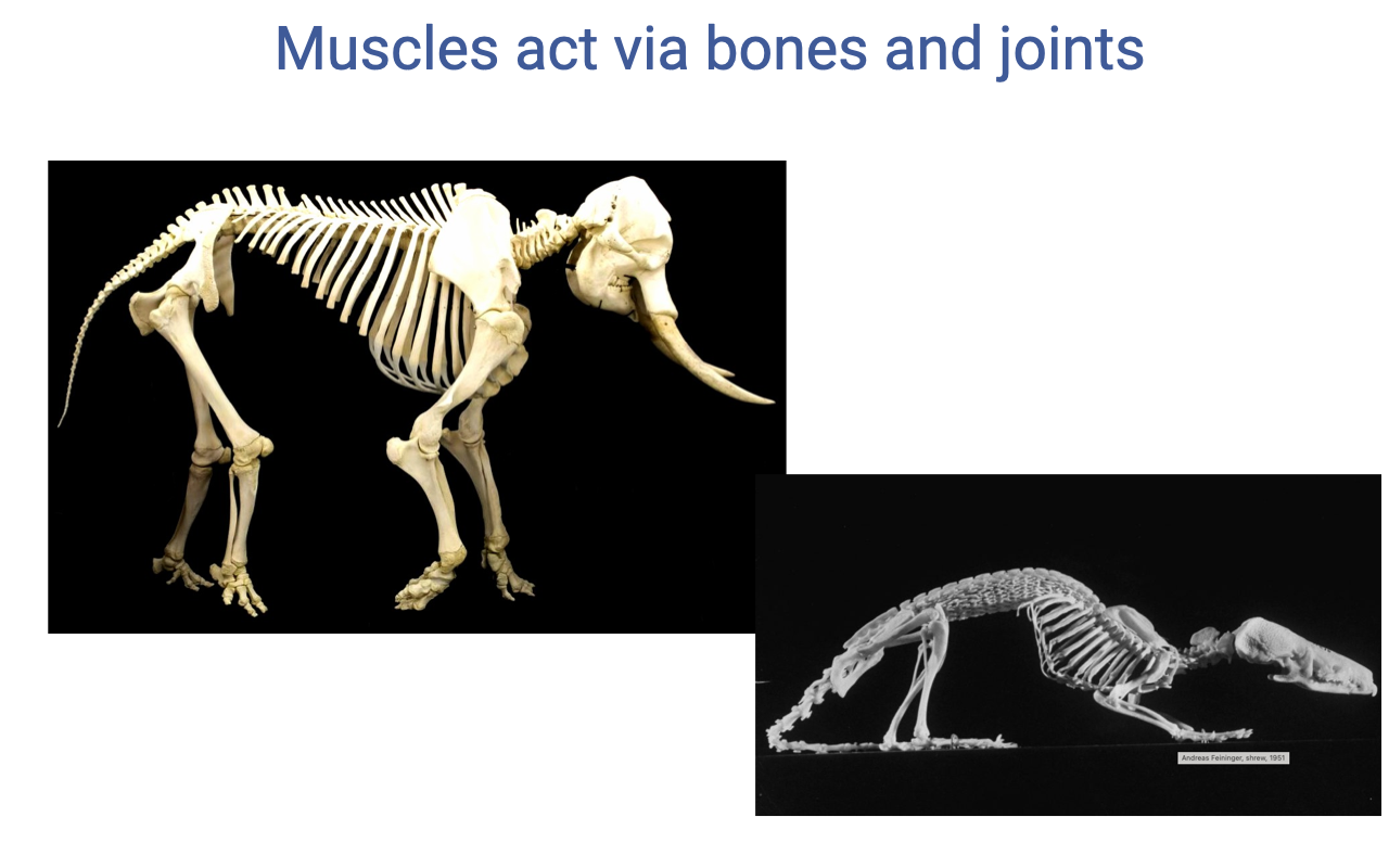
Why Skeletal Lever Systems Matter — Body Size
- Muscles do not act in isolation: they pull on bones that rotate around joints. The skeleton is the lever system through which muscle force becomes movement.
- Comparative observation: small animals (shrews, mice) have a crouched posture; large animals (elephants, rhinos) have a straight-legged, columnar (graviportal) posture.
- Understanding lever systems is necessary to explain why this posture shift exists — and why it has implications for muscle force, work, and energetic cost.
Slide 25
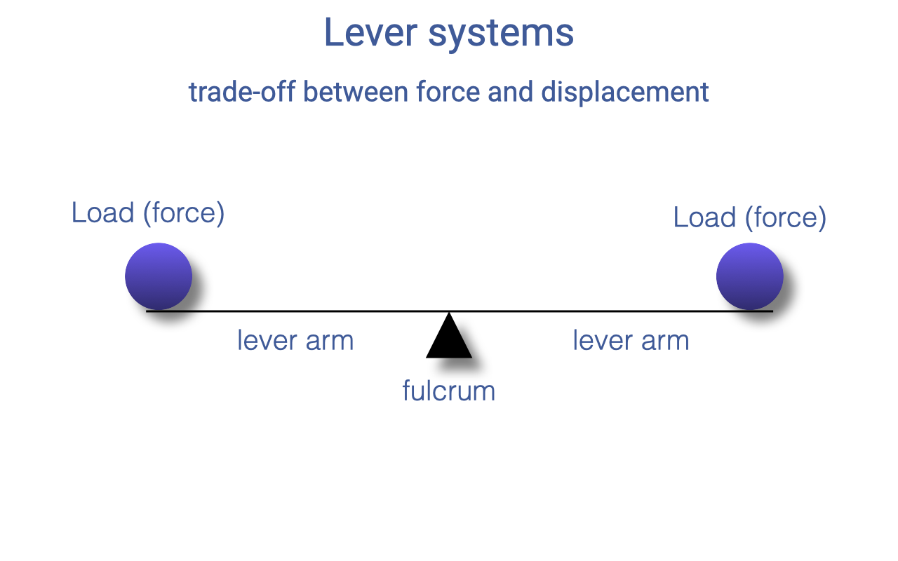
Lever Systems — The Basics
- A lever is a rigid bar that rotates around a fulcrum (the joint).
- Each load applies a force at some distance from the fulcrum — the lever arm (or moment arm).
- A lever can be balanced when the torques on both sides are equal — and the trade-off between force and displacement is built directly into the geometry.
Slide 26
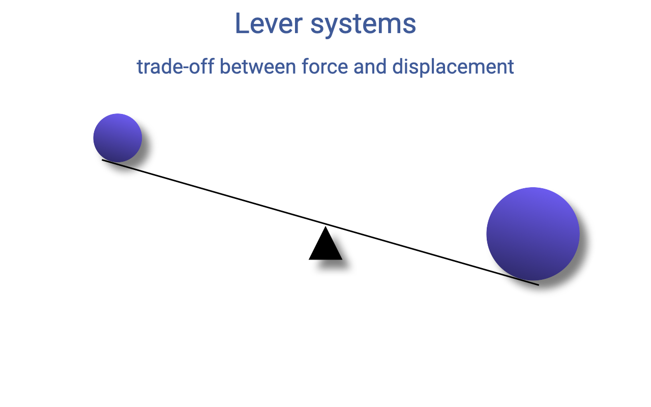
Imbalanced Loads — Lever Rotates Toward the Heavier Side
- When the torques on the two sides of a lever are not equal, the lever rotates toward the heavier side.
- A familiar example: on a playground seesaw, a heavier child sinks the seesaw toward themself.
- To rebalance the lever without removing the heavier load, you have to change the moment arm rather than the force itself.
Slide 27
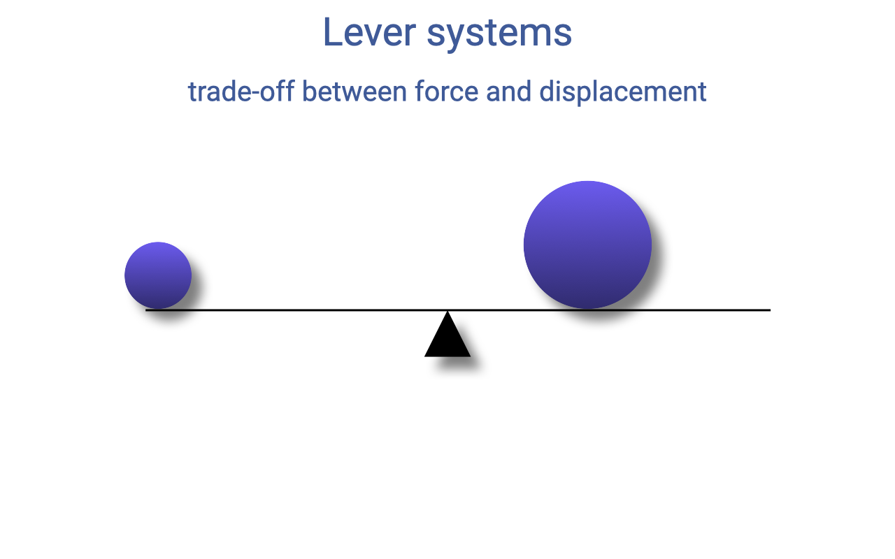
Balancing By Adjusting the Moment Arms
- The larger force can be balanced if it sits closer to the fulcrum — i.e., with a shorter moment arm.
- This is the basic intuition of a lever: a small force at a long lever arm can balance a large force at a short lever arm.
- The trade-off is between force and displacement: a small force traveling a large distance does the same total work as a large force traveling a small distance. Levers convert one currency to the other.
Slide 28
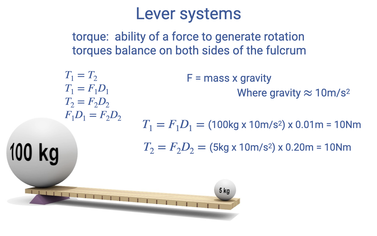
Torque Balance — Worked Example
- Torque ($T$) = the rotational effect of a force around a fulcrum:
- where $F$ is the force and $D$ is the perpendicular distance from the line of action of the force to the fulcrum.
- For a balanced lever:
- Worked example with g ≈ 10 m/s² for simplicity:
- 100 kg side: $T_1 = (100 \text{ kg} \times 10 \text{ m/s}^2) \times 0.01 \text{ m} = 10 \text{ N·m}$.
- 5 kg side: $T_2 = (5 \text{ kg} \times 10 \text{ m/s}^2) \times 0.20 \text{ m} = 10 \text{ N·m}$.
- Confirms balance: the 100 kg mass at 0.01 m balances the 5 kg mass at 0.20 m — short moment arm × large force = long moment arm × small force.
- Lever systems are passive — work in equals work out. They convert force to displacement (or vice versa) without adding or subtracting energy.
Slide 29
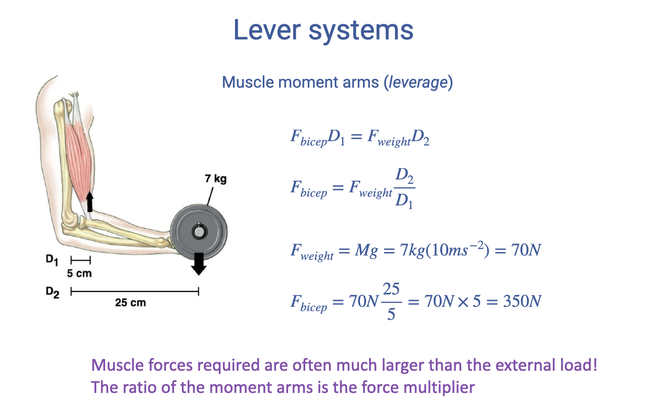
Applied — The Biceps Curl
- Biceps moment arm D1 ≈ 5 cm (insertion to elbow joint center).
- External-load moment arm D2 ≈ 25 cm (dumbbell to elbow joint center).
- For a 7 kg dumbbell:
- Muscle forces required to resist external loads are often many times larger than the external load itself — because muscles typically insert close to the joint while loads act far from the joint. The ratio of moment arms is the force multiplier.
- This force amplification is paid for by a corresponding displacement amplification at the load — small muscle shortening produces large hand motion.
Slide 30
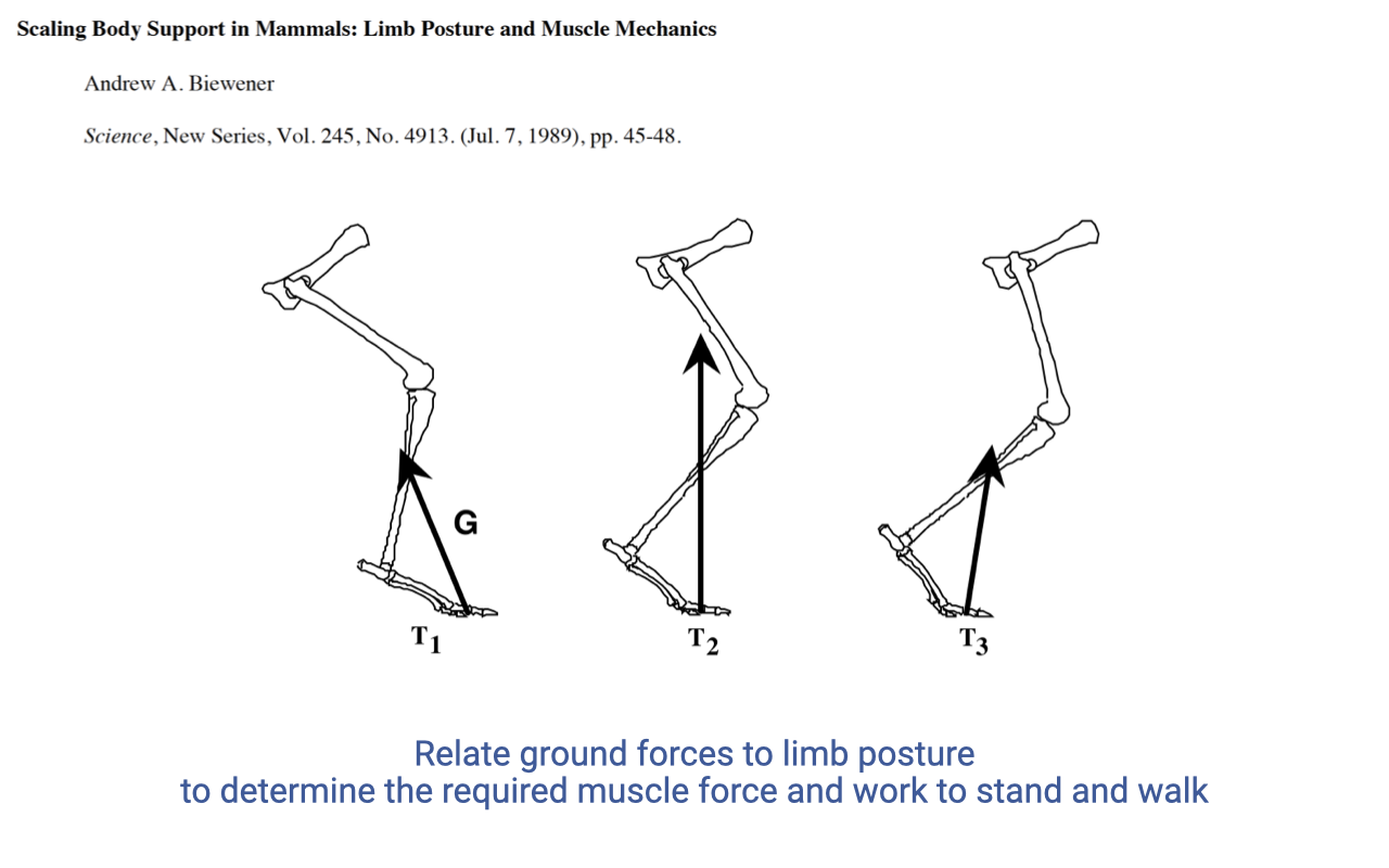
Biewener (1989) — Scaling of Body Support
- Classic comparative paper applying the lever-system concept across body sizes.
- In standing or walking, the ground reaction force (GRF) must support body weight. This GRF acts at some perpendicular distance from each joint center — the external moment arm — which depends on limb posture.
- The same GRF produces different muscle-force demands depending on whether the limb is crouched (long external moment arm) or upright (short external moment arm).
Slide 31
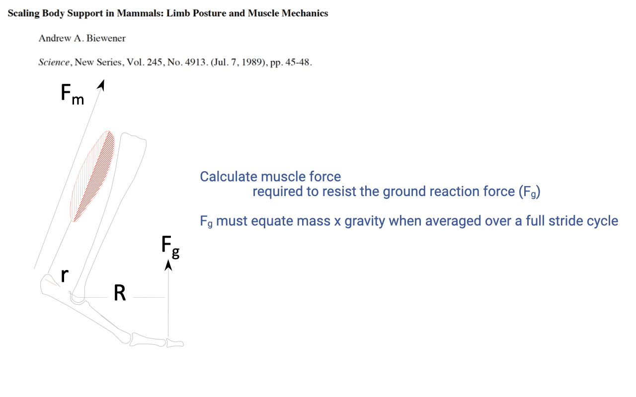
The Biewener Limb Lever System
- Fm = muscle force, acting at moment arm r (the muscle’s insertion-to-joint distance — primarily set by skeletal morphology).
- Fg = ground reaction force, acting at moment arm R (the perpendicular distance from the GRF vector to the joint center — primarily set by limb posture).
- Fg averaged over a full stride must equal body weight (mass × gravity) for an animal moving at steady speed.
Slide 32
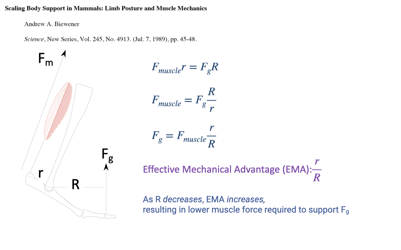
Effective Mechanical Advantage (EMA)
- Torque balance at the joint:
- Solving for muscle force:
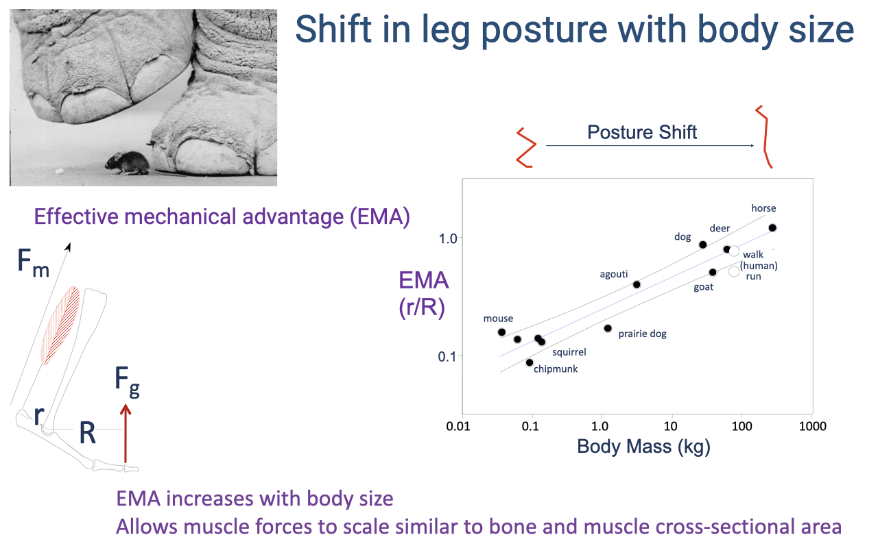
- The ratio r / R is the effective mechanical advantage (EMA):
- Higher EMA → lower muscle force required to support body weight.
- A straight (upright) limb posture keeps the GRF vector closer to the joint center → smaller R → higher EMA.
- This is why a straight-legged stance is energetically cheap — try standing with bent knees and you can feel the muscular effort rise immediately.
Slide 33
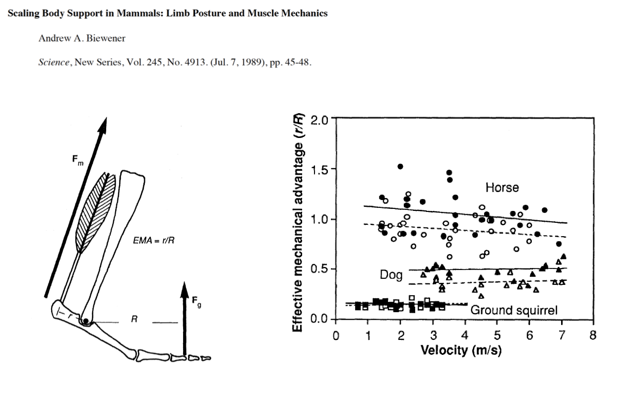
EMA Across Species — Larger Animals Have Higher EMA
- Across species (horse, dog, ground squirrel):
- EMA does not change much with running velocity within a species.
- EMA increases dramatically with body size: horse ~1.0, dog ~0.4–0.5, ground squirrel ~0.15–0.2.
- This means larger animals can produce body-weight-supporting forces with less mass-specific muscle force — they exploit a more upright posture to make their lever systems mechanically efficient.
Slide 34
Scaling of EMA With Body Size — Mammals
- EMA scales positively with body mass across mammals:
- Small animals (mouse, ~30 g): EMA ~0.1.
- Large animals (horse, ~500 kg): EMA ~1.0.
- The mechanism is a postural shift: larger animals adopt straighter limbs, which reduces R relative to r.
- This scaling allows muscle and bone forces to scale similarly to muscle and bone cross-sectional area — preventing large animals from breaking under their own weight (or needing impossibly disproportionate muscle masses).
- Humans are slightly off the mammalian regression: walking has a relatively high EMA (straight knee), but running EMA is lower (more flexed knee).
Slide 35
The Same Pattern in Birds — With High Within-Size Diversity
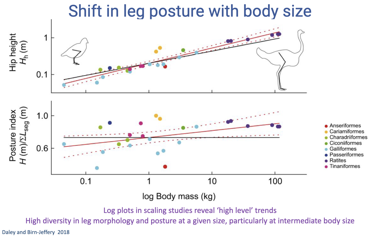
- Comparative study of 23 bird species (Daley and Birn-Jeffery 2018) shows the same trend of more upright posture with larger body size — the EMA scaling is not unique to mammals.
- Caveats to log-log scaling plots:
- They reveal high-level trends but average over substantial within-size diversity.
- At intermediate body sizes (~1 kg), the same body mass can have very different limb postures depending on locomotor ecology (e.g., ground-foragers vs. take-off-flight specialists).
- The scaling rules apply broadly, but selection for specific behaviors introduces species-specific deviations.
Slide 36
Ankle Moment Arm and Human Running Economy
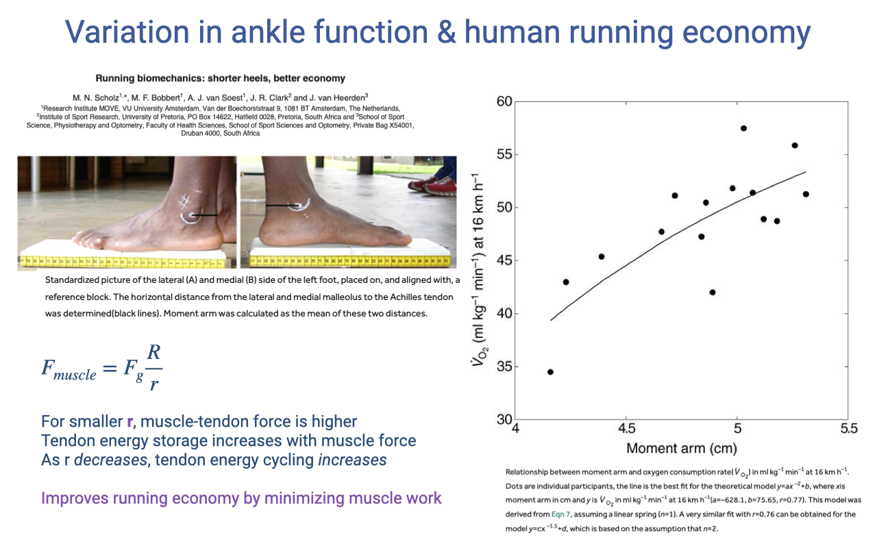
- Within humans (Scholz et al.), individual variation in ankle moment arm (Achilles tendon to ankle joint center) significantly predicts running economy:
- Shorter ankle moment arm → better running economy (lower V̇O2 at 16 km/h).
- Mechanism — counterintuitive at first:
- From the lever equation: smaller r → higher Fmuscle for a given Fg.
- But higher muscle–tendon force increases tendon strain energy storage in the Achilles tendon.
- The tendon’s elastic energy cycling can do work that the muscle would otherwise have to do — minimizing muscle work and improving economy.
- This is a preview of the integrative theme of Lecture 14: muscle, tendon, lever, and limb posture all act together to determine in vivo muscle function.
Slide 37
Learning Objectives — Recap
- Muscle morphology determines mechanical function: PCSA = volume / fiber length sets force capacity; fiber length sets displacement and velocity capacity; volume (mass) sets work and power. Tendon design (LT/Lo and AT/PCSA ratios) determines whether the MTU acts as a spring (economy, elastic cycling) or a direct-drive actuator (position control, range of motion).
- Lever-system equation: $F_{muscle} = F_g \times R/r$. Muscle forces required to support external loads are typically many times larger than the external loads themselves, because muscles insert close to the joint while loads act far from it.
- EMA scales positively with body mass across mammals and birds (mouse → horse). Larger animals adopt more upright postures — reducing R relative to r — so that mass-specific muscle and bone forces stay roughly constant despite increasing body size.
Key Equations
| Equation | Name | Description |
|---|---|---|
| $\sigma_{specific} = F / \text{PCSA} \approx 18\text{–}30 \text{ N/cm}^2$ | Specific tension | Force per unit physiological cross-sectional area; highly conserved across vertebrates and varies modestly with fiber type. A typical value of ~25 N/cm² is used as an estimate. |
| $\text{PCSA} = \dfrac{\text{Volume}}{\text{fiber length}}$ | Physiological cross-sectional area | The cross-sectional area of muscle perpendicular to the fibers; used to compute maximum force capacity. Volume is obtained from mass × density (~1.06 g/cm³) or imaging. |
| $F_{max} \propto \text{PCSA}$ | Force capacity | Maximum force is proportional to the number of sarcomeres in parallel — i.e., the PCSA. |
| $\text{Displacement}, V_{max} \propto L_{fiber}$ | Displacement and velocity capacity | Maximum shortening distance and maximum shortening velocity are proportional to the number of sarcomeres in series — i.e., the fiber length. |
| $\text{Work}, P \propto \text{Volume} = \text{PCSA} \times L_{fiber}$ | Work and power capacity | Maximum work and power are proportional to the muscle’s volume (or, equivalently, mass via the conserved muscle density). |
| $T = F \times D$ | Torque | The rotational effect of a force around a fulcrum, where $D$ is the perpendicular distance from the force’s line of action to the fulcrum. |
| $F_1 D_1 = F_2 D_2$ | Lever balance | Torques on either side of a fulcrum balance at equilibrium. |
| $F_{muscle} = F_g \times \dfrac{R}{r}$ | Limb lever equation | Muscle force required to resist the ground reaction force, where r is the muscle’s moment arm (skeletal morphology) and R is the GRF moment arm (set by posture). |
| $\text{EMA} = \dfrac{r}{R}$ | Effective mechanical advantage | Ratio of muscle moment arm to GRF moment arm. Higher EMA → lower required muscle force per unit body weight; scales positively with body mass across vertebrates. |
Glossary of Key Terms
| Term | Definition |
|---|---|
| Hill-type properties | The intrinsic isometric force–length and isotonic force–velocity relationships of muscle, named after A.V. Hill, who developed the experimental methods to measure them. |
| Musculoskeletal model | A computational model of the body that combines bones, joints, and Hill-type muscle elements to predict in vivo muscle force from observed motion (e.g., OpenSim). |
| B-mode ultrasound (in muscle) | Non-invasive imaging method used in human studies to measure fascicle length and pennation angle in real time during contraction. |
| Dynamometer | A rigid device that fixes joint angle and measures resulting joint torque during a maximal contraction; the human equivalent of a muscle ergometer. |
| Fiber arrangement | The geometric organization of muscle fibers within a muscle belly: parallel (longitudinal), pennate (unipennate, bipennate), or multipennate. |
| Pennation angle | The angle between the muscle fibers and the line of action of the muscle–tendon unit. Increasing pennation packs more fibers per unit volume. |
| Fascicle / fiber length (Lfiber) | The length of a muscle fascicle (a bundle of fibers). Determines the displacement and velocity capacity of the muscle. |
| Physiological cross-sectional area (PCSA) | The cross-section of muscle perpendicular to the fibers, computed as volume / fiber length. Determines the muscle’s maximum force capacity. |
| Specific tension (σ) | Force per unit physiological cross-sectional area; ~18–30 N/cm² across vertebrate skeletal muscle, highly conserved with modest fiber-type variation. |
| Aponeurosis | The flat, broad internal tendon that lies on (or within) the muscle belly and connects to the external tendon. Part of total tendon length LT. |
| External tendon | The free portion of the tendon that connects the muscle to bone (e.g., the visible Achilles tendon). |
| Tendon slack length (LT) | The length of the tendon (aponeurosis + external) at zero force; one of the key architectural parameters. |
| LT/Lo ratio | Ratio of tendon slack length to optimal muscle fiber length. High (long tendon, short fibers) → economic force, elastic energy cycling. Low (short tendon, long fibers) → range of motion and position control. |
| AT/PCSA ratio | Ratio of tendon cross-sectional area to muscle PCSA; sets the stiffness of the tendon relative to the force the muscle can apply. Low AT/PCSA → compliant tendon, high elastic energy cycling. |
| Compliant tendon | A tendon that stretches substantially under physiological loads; stores and returns elastic strain energy. Low AT/PCSA. |
| Stiff tendon | A tendon that stretches little under load; transmits force directly to rotate the joint. High AT/PCSA. |
| Concentric contraction | Shortening contraction (Fmuscle > load); positive work; via the F–V relation, higher velocity demands a higher volume of active muscle. |
| Eccentric contraction | Lengthening contraction (Fmuscle < load); negative work; lower volume of active muscle and lower ATP per unit force, but highest injury risk. |
| Isometric contraction | No length change at the joint level; force only, to resist the load; cost is steady-state proportional to force, with frequency contributing in cyclic contractions. |
| Lever system | A rigid bar (bone) that rotates around a fulcrum (joint), with forces applied at perpendicular distances called moment arms. |
| Fulcrum | The pivot point of a lever — at the joint center of rotation in musculoskeletal systems. |
| Moment arm (lever arm) | The perpendicular distance from the line of action of a force to the fulcrum; determines that force’s torque. |
| Torque (T) | Rotational effect of a force, $T = F \times D$. Measured in newton-meters (N·m). |
| Muscle moment arm (r) | The perpendicular distance from the muscle’s line of action to the joint center; determined primarily by skeletal morphology (e.g., calcaneal length for the Achilles tendon at the ankle). |
| External (GRF) moment arm (R) | The perpendicular distance from the ground reaction force vector to the joint center; determined primarily by limb posture. |
| Effective mechanical advantage (EMA) | The ratio r/R. Higher EMA means lower required muscle force to support a given GRF. Scales positively with body mass across mammals and birds. |
| Inverse dynamics | A technique for inferring muscle and joint forces from external measurements of motion (motion capture or high-speed video) and ground reaction force. Requires lever-system analysis at each joint. |
| Graviportal posture | The straight-legged, columnar limb posture seen in very large animals (elephants, rhinos), maximizing EMA to keep muscle forces tractable despite large body weight. |
| Crouched posture | The flexed-limb posture seen in small animals (mice, shrews) and in humans during deep knee bends; lower EMA, higher muscle-force demand. |