Week 6 Friday Review and Discussion

19 slides

Slide 1

Friday review and discussion session for Week 6: Integrative Muscle Structure and Function — Organ, Limb, and Whole-Organism Levels.
Wraps up content from Wednesday’s lecture on whole-organism muscle function (case studies in turkey, wallaby, guinea fowl, cockatiel) and links it to human walking, running, and assistive-device design.
Closes with a structured practice-question segment to prepare for the weekly quiz, covering muscle architecture (cheetah vs greyhound), the lever-system equation in a static squat, and the work-loop diagram as a graphical tool.

Slide 2

Announcement — Godoy Fellowship in Movement Sciences

The Dr. M. Marlene Godoy Fellowship in Movement Sciences is a new summer research fellowship administered by the UCI Center for Integrative Movement Sciences (CIMS).
Award: $4,000 stipend for 10 weeks of intensive summer research; expects to fund about two fellows in 2026.
Eligibility: UCI undergraduates with a confirmed faculty sponsor working in movement physiology, biomechanics, motor learning, rehabilitation, or a related area.
How to apply: Application form linked from the QR code on the slide and at https://cims.uci.edu/call-for-godoy-fellows-2026/. To find a sponsor, the recommended path is to browse CIMS-affiliated faculty at cims.uci.edu and contact labs directly — funding makes faculty more likely to take on a student.
Background: Dr. Marlene Godoy is a UCI biology alumna (~1976) who became a successful dentist and endowed this fellowship to support undergraduate research experiences.

Slide 3

Distal Hindlimb Muscles and the Economy of Minimizing Work

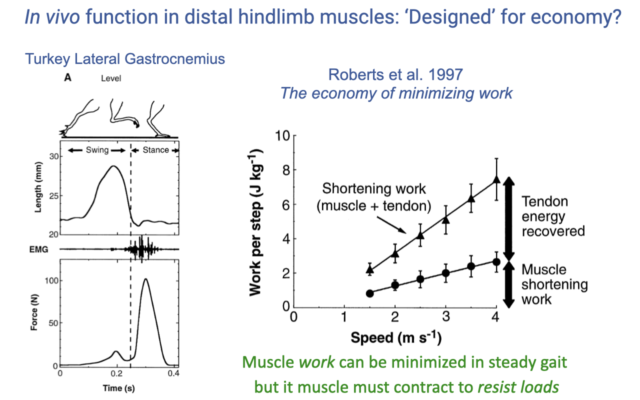
Roberts et al. 1997 is one of the earliest direct in vivo measurements of an individual muscle during locomotion. Used turkeys (an effective ground bird) because the turkey gastrocnemius has architecture similar to humans and guinea fowl.
They implanted sonomicrometry crystals in the muscle (to measure fascicle length) and a tendon force buckle (to measure muscle-tendon force) — direct measurements that the joint-level analysis cannot give.
During level running, the time traces show:
- Swing phase: passive stretch with only a small force blip (passive connective-tissue stretch).
- Stance phase: muscle activates just before foot contact and develops a force peak — its main job is to support body weight against gravity.
- Length stays nearly constant during force development → isometric contraction at the muscle level.
The right-hand plot shows that as running speed increases, the total ankle “shortening work” estimated from inverse dynamics rises steeply, while muscle shortening work rises only modestly — the difference is the elastic energy cycled in the tendon.
More than half of the apparent ankle work is delivered by tendon recoil, not muscle shortening — a major savings because shortening muscle uses much more energy than isometric muscle.
Muscle work can be minimized in steady gait, but the muscle still has to be turned on to resist loads. This is why metabolic cost in steady locomotion is well predicted by force demand, not work demand.

Slide 4

Diversity of In Vivo Ankle Extensor Muscle Dynamics

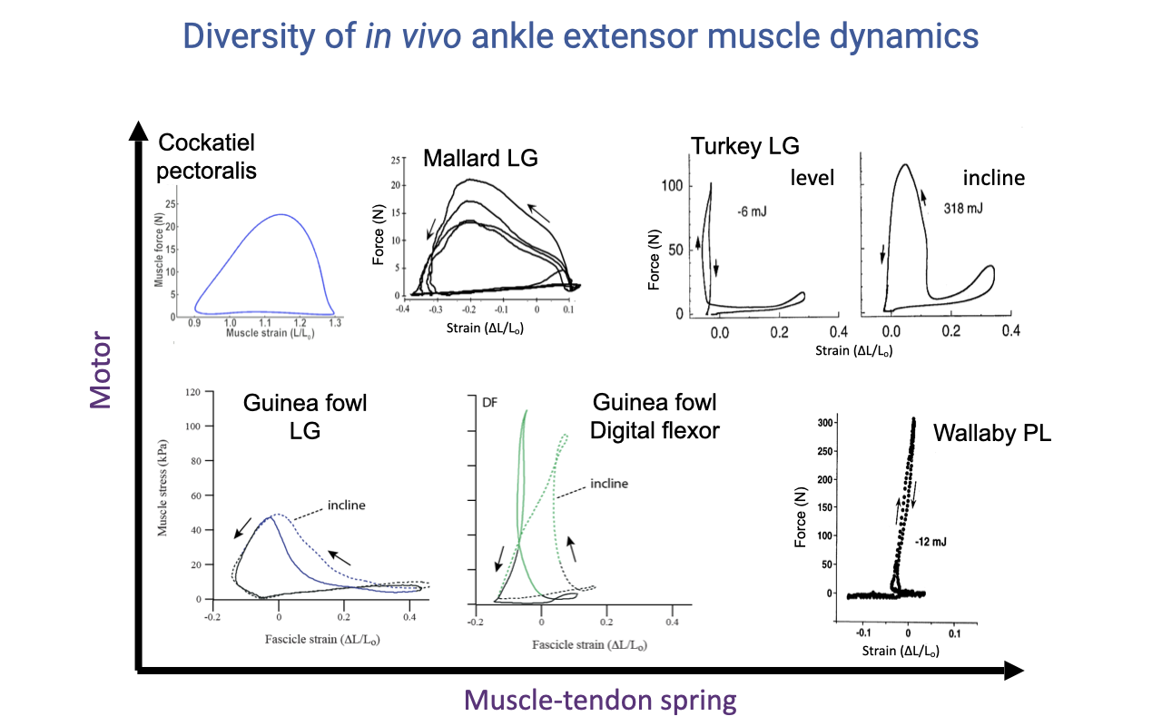
A unifying view of all the case studies from Wednesday’s lecture, plotted as a 2D space with muscle-tendon spring function on one axis and motor (positive-work) function on the other.
Motor specialists (top-left): the cockatiel pectoralis powers the downstroke in flight with very large positive work loops; nearly identical shape across speeds and conditions — designed for one job.
Mallard lateral gastrocnemius is also motor-like — specialized for propulsion during swimming.
Turkey lateral gastrocnemius is multifunctional:
- Level running: narrow vertical L-shape ≈ near-isometric, ~−6 mJ (essentially zero work) → acts as a strut allowing the tendon to act as a spring.
- Incline running: same muscle activates earlier, shortens substantially while developing force, and produces ~318 mJ of positive work → switches to motor mode when the task demands it.
Guinea fowl lateral gastrocnemius is a generalist — does positive work even on level ground, with extra work on inclines and especially on uneven terrain (see Lecture 14, Slides on stumble recovery).
Guinea fowl digital flexor is an energy absorber (net negative work loop) — cushions impact at heel-strike.
Spring specialists (bottom-right): the wallaby plantaris has such an extreme architecture (very long, thin tendon and very short fascicles) that it can essentially only act as a spring; even on inclines, the muscle does almost no positive work and all of the propulsive power comes from the proximal muscles at the hip.
Morphology constrains function — the more specialized the architecture, the more constrained the role; versatility costs specialization. The turkey gastrocnemius retains versatility because it has more moderate architectural specialization.

Slide 5

Proximo-Distal Distribution of Muscle Mass

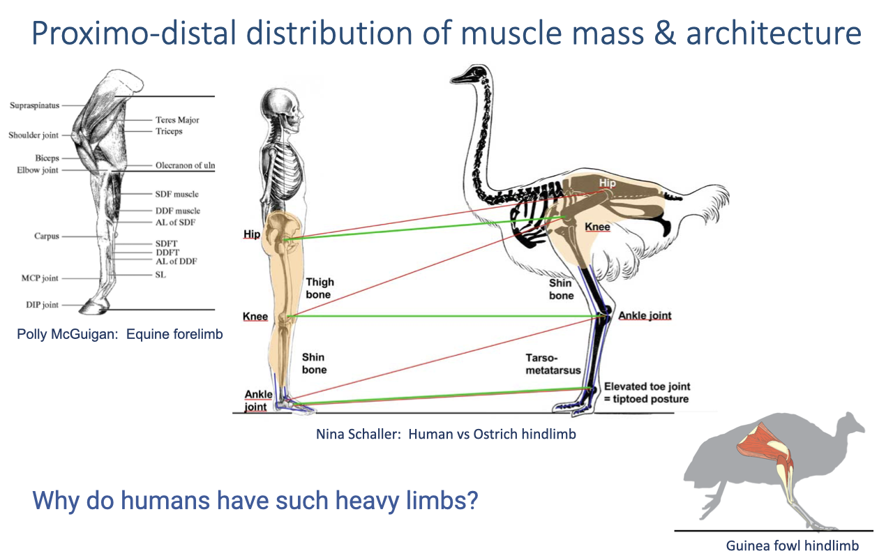
General pattern across cursorial animals: high-mass muscles concentrated proximally (at the shoulder or hip), specialized short-fibered muscles with long tendons distally.
Why this gradient? Distal mass is disproportionately costly to oscillate during swing (think ankle weights vs hip weights at the gym). A heavy distal limb increases the moment of inertia about the hip and so the work needed each step.
Specialized cursors (ostrich, horse) take this to the extreme — they stand on their toes with tarsals/metatarsals elongated into a third leg segment, and their distal limbs are mostly tendon and bone with little muscle.
Humans are anomalously heavy-legged: we are excellent endurance runners but mediocre sprinters compared to other mammals our size, and we have substantial muscle mass distally (calf and foot intrinsics) along with a plantigrade posture (flat-footed).
Our femur is elongated relative to our ancestors, but the distal limb is not — the opposite of the cursorial mammal pattern. This unusual arrangement is an active question in anthropology and human biomechanics — likely tied to upright bipedal walking and endurance running rather than maximum top speed.
The recurring question across this lecture: why do humans have such heavy distal limbs, and what is that good for? Returns at the end of the within-species comparison (Slide 6) and in human walking ultrasound (Slide 10).

Slide 6

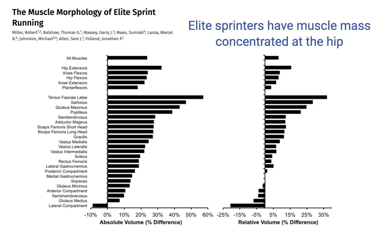
Within-Species Variation — Elite Sprinters Concentrate Mass at the Hip

Miller et al. compared elite sprint runners to sub-elite sprinters running the same distances. Elite sprinters had about 20% higher overall hindlimb muscle mass in absolute terms.
More striking: the relative-volume distribution is shifted proximally:
- Largest relative gains in the hip extensors (gluteus maximus, biceps femoris long head, adductor magnus, semitendinosus) and other proximal muscles like tensor fasciae latae and sartorius.
- Distal muscles (soleus, lateral compartment) actually show smaller relative volume — they are not what distinguishes elite sprinters.
Why this distribution? Sprint performance is dominated by the rate of positive power production for acceleration, and that power comes from the hip extensors. Concentrating mass proximally also keeps distal limb inertia low, so the leg can be cycled quickly during fast strides.
This is the same proximo-distal logic seen across species (Slide 5), now operating within humans as a marker of running specialization.
Human distal-limb morphology is an outlier compared with cursorial mammals, but even within humans, sprinters look more “ostrich-like” in their proximal mass concentration than the average person.

Slide 7

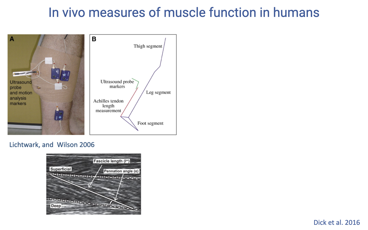
In Vivo Ultrasound + Motion Capture in Humans

The same direct-measurement logic that motivated the turkey study is now feasible in walking and running humans using non-invasive B-mode ultrasound combined with motion capture.
Set-up:
- Ultrasound probe strapped over the medial gastrocnemius (or soleus) records fascicle length and pennation angle in real time.
- Motion-capture markers on thigh, leg, and foot segments give the joint kinematics, from which Achilles tendon length can be reconstructed (whole muscle-tendon unit length minus fascicle projection along the line of action).
The B-mode ultrasound image at the bottom shows the superficial and deep aponeuroses with the fascicles running diagonally between them at a measurable pennation angle (α) — this is the same architectural picture from Lecture 13, now visible in a living, walking human.
This is the only way to separate fascicle behavior from tendon behavior in humans. The MTU length comes from joint kinematics; the fascicle length comes from ultrasound; the tendon length is the difference — and the difference is what reveals elastic energy storage in the Achilles.
Develops the same concept as the turkey sonomicrometry study (Slide 3), but applied to humans where surgical implantation is not possible.

Slide 8

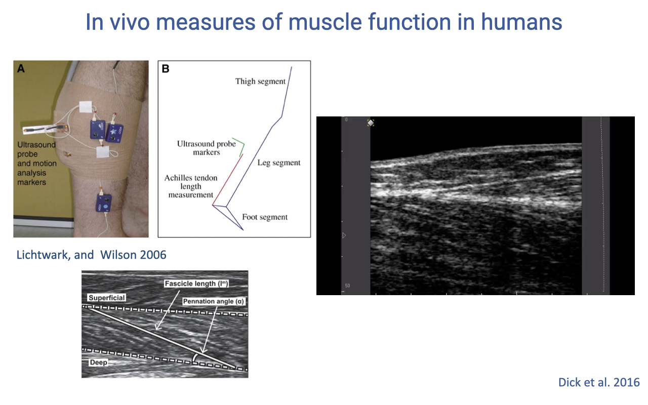
Reading the Ultrasound Frame During Gait

Same set-up as Slide 7 — emphasis here is on the dynamic ultrasound clip that is recorded during a stride: pennation angle and fascicle length change frame-by-frame as the muscle activates and the joint rotates.
During the loading response of stance, the MTU lengthens but the fascicle lengthens only slightly — most of the stretch is taken up by the Achilles tendon, exactly the same pattern observed in vivo in the turkey gastrocnemius (Slide 3).
During push-off, the MTU shortens rapidly while the fascicle shortens only modestly — the difference is tendon recoil, returning stored elastic energy to power propulsion.
A single ultrasound frame is uninformative — you need the time-series across the stride to see the decoupling of fascicle and MTU motion. This is the technique that finally let researchers verify in humans the strut-and-spring mechanism Roberts et al. described in turkeys.

Slide 9

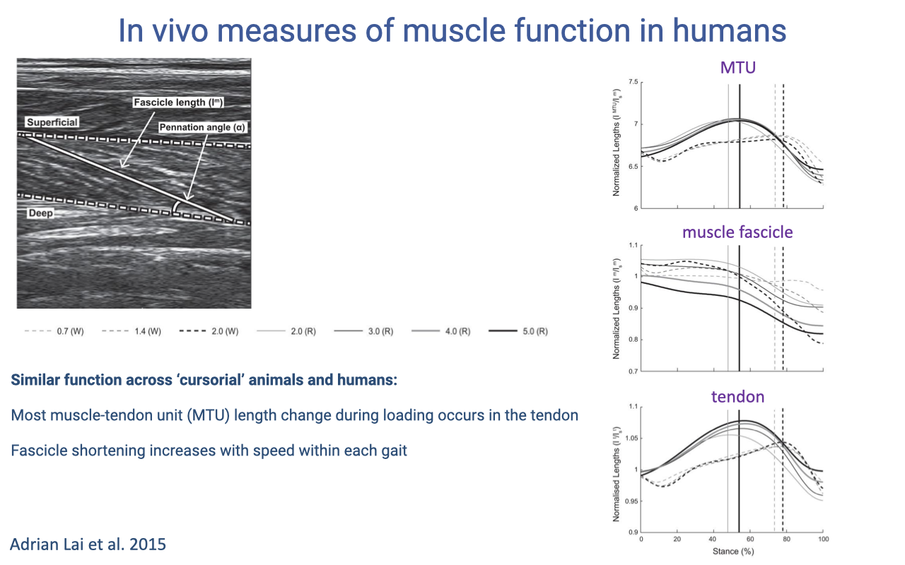
Decoupling of MTU, Fascicle, and Tendon Length Across Speeds

Three normalized plots (Lai et al. 2015) over one stride for the human medial gastrocnemius across walking and running speeds:
- MTU: large length excursion that grows with speed.
- Muscle fascicle: relatively flat — fascicle shortens modestly, and the magnitude does increase with speed but stays much smaller than the MTU excursion.
- Tendon: large excursion that mirrors the MTU — most of the loading stretch happens here.
Across cursorial animals and humans, the majority of MTU length change during loading is taken up by the tendon, not the fascicle. This is the strut-and-spring mechanism confirmed in the human gastrocnemius.
As gait speed rises within walking or within running, the fascicle shortening increases modestly — the muscle does more active work at higher speeds, while the tendon continues to do most of the elastic energy cycling.
Re-reinforces the conceptual point from Slide 3: muscle work is not the same as joint work because tendon compliance decouples them. You cannot infer muscle behavior from joint kinematics alone.

Slide 10

Soleus Operating Point and the Walk-to-Run Transition

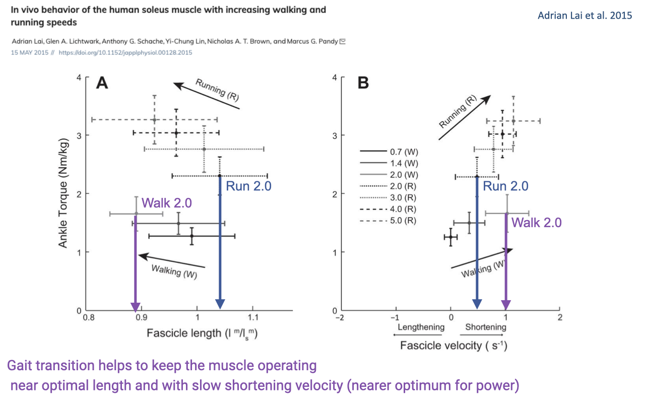
Lai et al. measured soleus fascicle length and velocity across walking (0.7, 1.4, 2.0 m/s) and running (2.0, 3.0, 4.0, 5.0 m/s) speeds — including matched 2.0 m/s in both gaits.
Panel A (length-torque): at the same 2.0 m/s, walking puts the soleus at a shorter, less-optimal fascicle length with lower ankle torque; switching to running at the same speed shifts the operating point to a longer fascicle length and higher ankle torque — closer to the plateau of the F–L curve.
Panel B (velocity-torque): walking at 2.0 m/s puts the muscle at a higher shortening velocity; running at the same speed puts it at a slower shortening velocity — closer to the velocity for peak power on the F–V curve.
The gait transition is partly a strategy to keep the soleus operating near optimal length and at slow shortening velocity — both more favorable for power production and for economy than walking quickly would be.
Connects directly to the F–L and F–V curves of Week 5 and the power–velocity practice problem (Week 5 Friday review): the body chooses gaits, in part, to keep the working muscle near the peak-power region of the F–V curve.

Slide 11

Applications — Prosthetic Running Blades

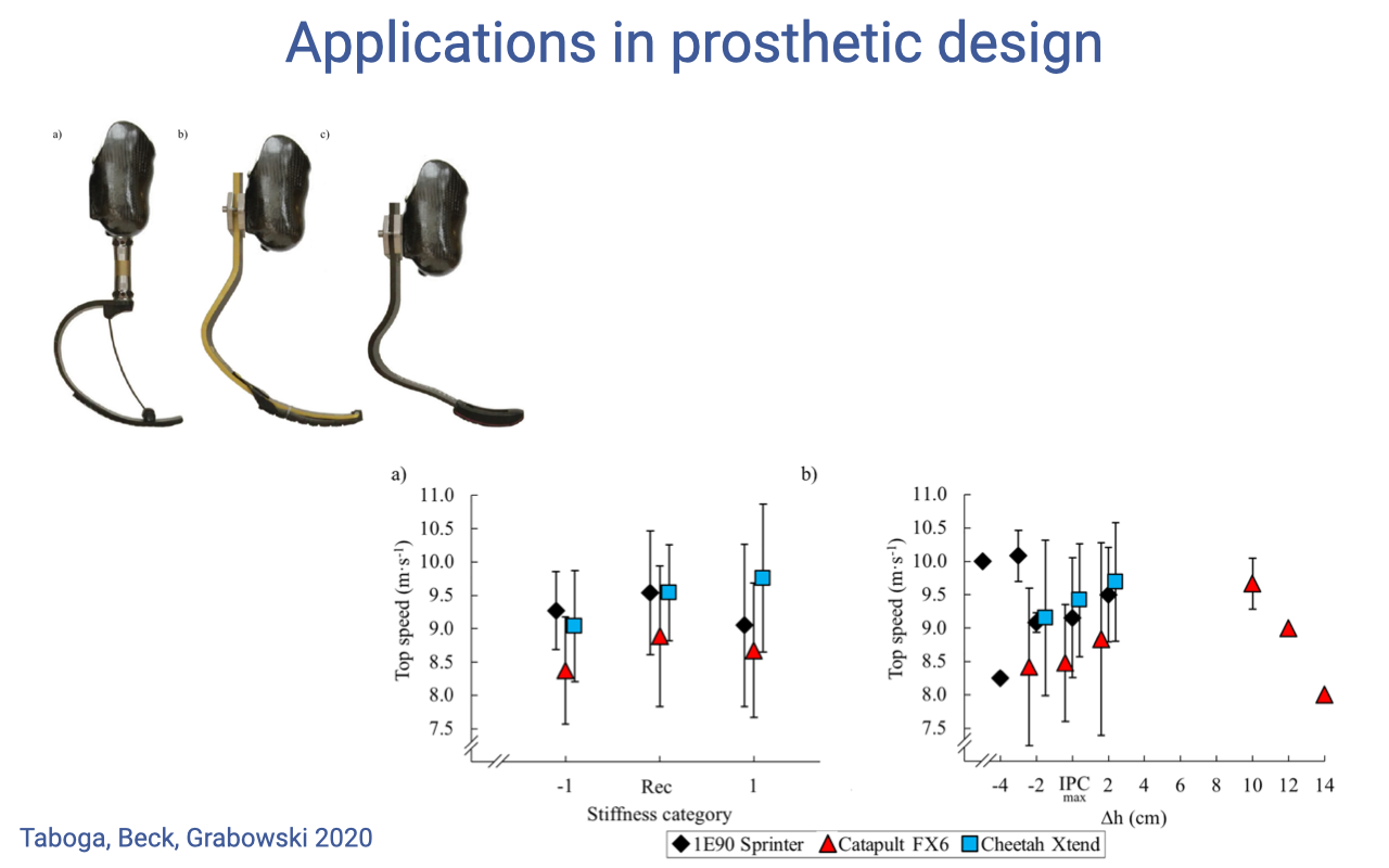
A direct application of muscle-tendon spring principles: carbon-fiber running blades are designed as passive elastic elements that store and recoil energy at heel-strike, mimicking the Achilles tendon in the intact human limb.
Taboga, Beck, and Grabowski (2020) tested whether stiffness category or height (Δh) of three commercial running blades (1E90 Sprinter, Catapult FX6, Cheetah Xtend) systematically affected top sprint speed in athletes with unilateral transtibial amputation.
There is no clear optimal stiffness across athletes — the within-blade variation is large, and the across-blade differences are modest. Different runners do best with different blade-stiffness combinations.
This mirrors a deeper biomechanical truth: even in intact humans, the best soleus-tendon stiffness for running depends on body mass, leg geometry, and stride preferences. There is no one-size-fits-all “optimal” tendon — and the same is true for prosthetic springs.
Blade design should be individualized to the athlete, the same way training programs are. The principles of muscle-tendon function (Lecture 14) inform the design space, but the fitting is empirical.

Slide 12

Applications — Ankle Exoskeleton Control (Set-up)

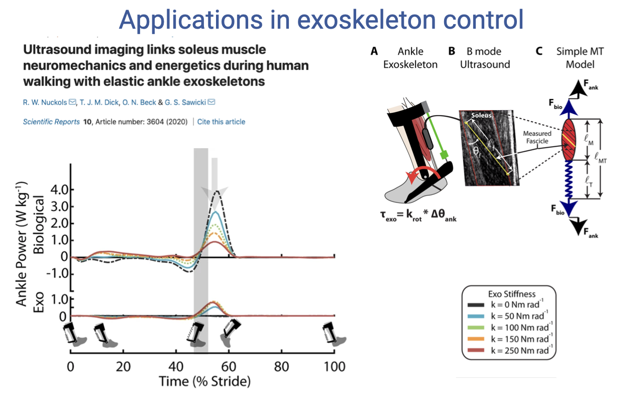
Nuckols et al. 2020 combined a passive elastic ankle exoskeleton with B-mode ultrasound to test how exoskeleton stiffness affects the biological soleus during walking.
Three measurements per condition:
- (A) Ankle exoskeleton with adjustable rotational stiffness (in series with the Achilles).
- (B) Synchronized B-mode ultrasound of the medial gastrocnemius/soleus to track fascicle behavior during the stride.
- (C) A simple muscle-tendon model that uses force balance to interpret the data: the exoskeleton, biological tendon, and muscle act in parallel and series as a coupled system.
The top-left plot shows the ankle power profile across one stride for the biological ankle vs. with the exoskeleton — the exoskeleton reshapes the timing and magnitude of ankle power output.
An exoskeleton spring that is too stiff unloads the muscle so much that it operates at sub-optimal length/velocity and has to develop more force, not less, at metabolic cost. A spring that is too compliant does too little work. There is a tuned optimum.

Slide 13

Applications — Tuning Stiffness Matters

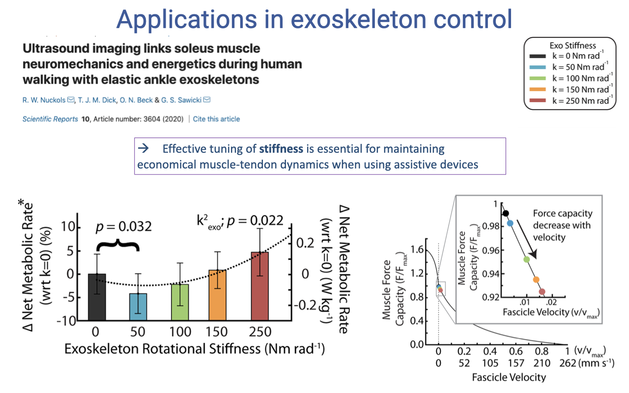
Nuckols et al.’s key result: net metabolic rate during walking depends on exoskeleton stiffness in a non-monotonic way (p = 0.032). Walking gets easier as stiffness rises from zero up to an intermediate value, then harder as stiffness rises further.
The mechanism (right inset): increasing exoskeleton stiffness changes the operating point of the soleus on its F–V curve:
- Zero/low stiffness: muscle works hard against the full ankle torque — high metabolic cost.
- Intermediate stiffness: muscle is partially unloaded → operates at a slower shortening velocity with higher force capacity → lower volume of active muscle for the same task → lower metabolic cost.
- Too-high stiffness: muscle is held nearly isometric at a length where its force capacity is low; it has to co-contract to maintain joint stability → higher metabolic cost again.
Effective tuning of stiffness is essential for maintaining economical muscle-tendon dynamics when using assistive devices.
A passive spring is not “free” energy — it changes the operating point of the muscle on its intrinsic F–L and F–V curves. Optimal device design requires understanding the biological muscle’s mechanical properties as well as the device.

Slide 14

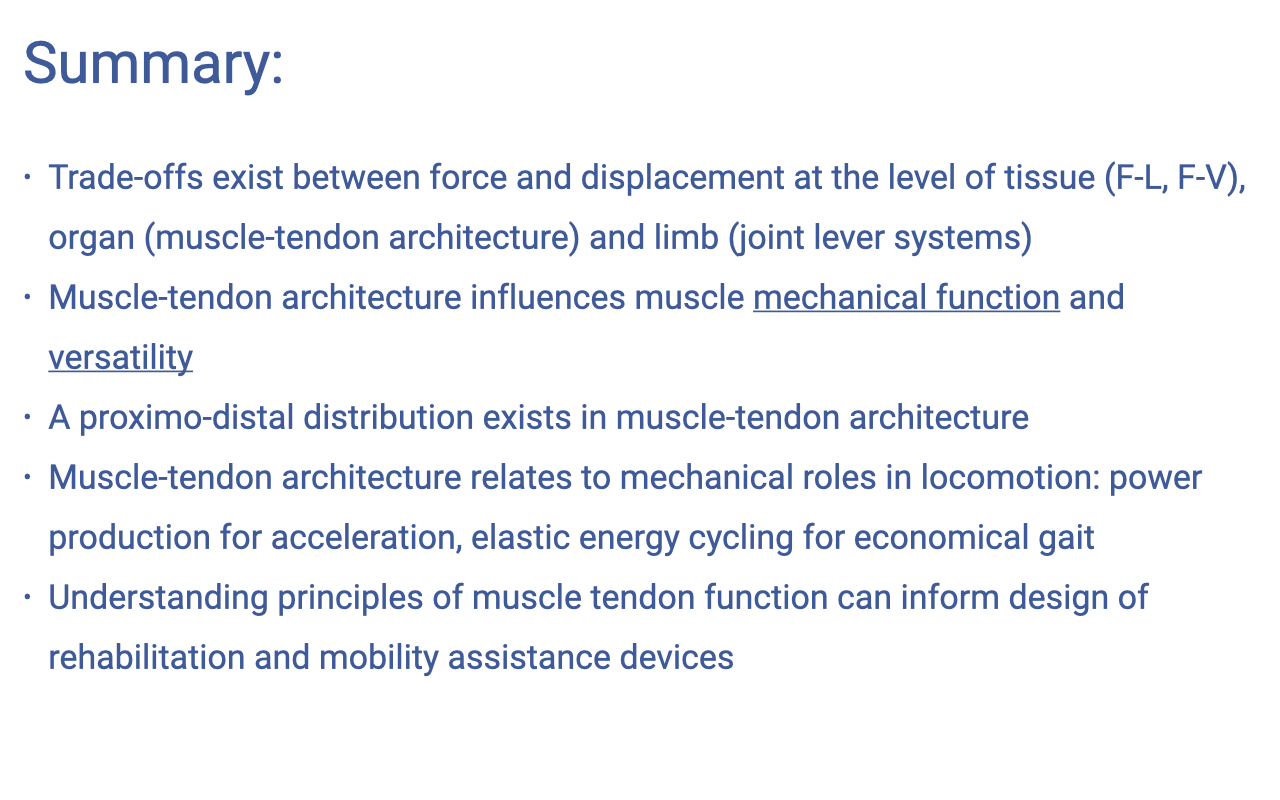
Summary of Lecture-Material Recap

Trade-offs at every scale of organization:
- Tissue (cellular and fiber): F–L and F–V curves — force vs displacement and force vs velocity.
- Organ (muscle architecture): PCSA vs fiber length, parallel vs pennate, tendon length and stiffness.
- Limb (lever systems): in-lever vs out-lever, effective mechanical advantage (EMA), force-velocity ratios at the joint.
Architecture-to-function mapping:
- Long fibers, low pennation, short stiff tendon → motor (cockatiel pectoralis, mallard LG).
- Short fibers, high pennation, long compliant tendon → spring (wallaby plantaris, horse distal limb).
- Intermediate architecture → multifunctional or generalist (turkey LG, guinea fowl LG).
Proximo-distal gradient is a whole-organism consequence: power-producing motors at the hip, springs at the ankle.
Locomotor roles map onto this gradient: acceleration and incline require positive power (proximal motors); steady gait is dominated by elastic energy cycling (distal springs).
Practical applications: prosthetic blades (Slide 11) and exoskeletons (Slides 12–13) succeed when their mechanical impedance matches the muscle-tendon roles they replace or augment.

Slide 15

Slide containing only the heading "Practice questions" centered on a white background in large blue text.

Transition — Practice-Question Section

Section divider — the remainder of the deck is structured as three practice questions designed to consolidate Week 6 content and prepare for the weekly quiz.
The questions test three different scales of muscle-tendon analysis:
1. Organ-level architecture — comparing two PCSA-and-fiber-length combinations (cheetah vs greyhound gastrocnemius).
2. Limb-level lever systems — quadriceps force in standing vs static squat.
3. In vivo dynamics — sketching three idealized work-loop shapes for isometric, positive-work, and negative-work contractions.

Slide 16

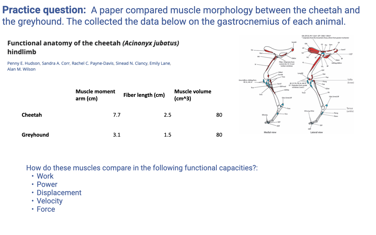
Practice Question 1A — Cheetah vs Greyhound Gastrocnemius Morphology

Setup: comparable-mass cursorial mammals (cheetah and greyhound) with very different running specializations. Both have gastrocnemius muscle volume = 80 cm³ but differ in moment arm and fiber length.

	Cheetah	Greyhound
Moment arm (cm)	7.7	3.1
Fiber length (cm)	2.5	1.5
Muscle volume (cm³)	80	80

Reasoning framework (revisit Lecture 13 architecture relationships):
- PCSA = Volume / Fiber length → higher for shorter fibers (greyhound) at fixed volume.
- Force capacity ∝ PCSA → greyhound gastroc has higher force capacity per unit volume.
- Maximum shortening velocity ∝ fiber length (number of sarcomeres in series) → cheetah gastroc has higher V_max at the muscle level.
- Maximum displacement ∝ fiber length → cheetah gastroc can shorten farther.
- Power = F × V. With volume fixed, power capacity is the same for both at the muscle level (volume sets the total power-producing tissue). But the operating range of velocities differs — cheetah operates over higher velocities, greyhound over lower velocities.
- Joint-level comparison must account for the moment arm: cheetah has a larger moment arm (7.7 vs 3.1 cm), so it produces more joint torque for a given muscle force, but with less angular displacement for a given fiber shortening. Greyhound is the opposite — small moment arm gives higher joint angular velocity at the cost of joint torque.
Qualitative summary:
- Cheetah: longer fibers + larger moment arm → designed for high-velocity, high-torque power output during sprinting acceleration.
- Greyhound: shorter fibers + smaller moment arm → designed for higher angular velocities at the joint at lower force, more like a distance runner.

Slide 17

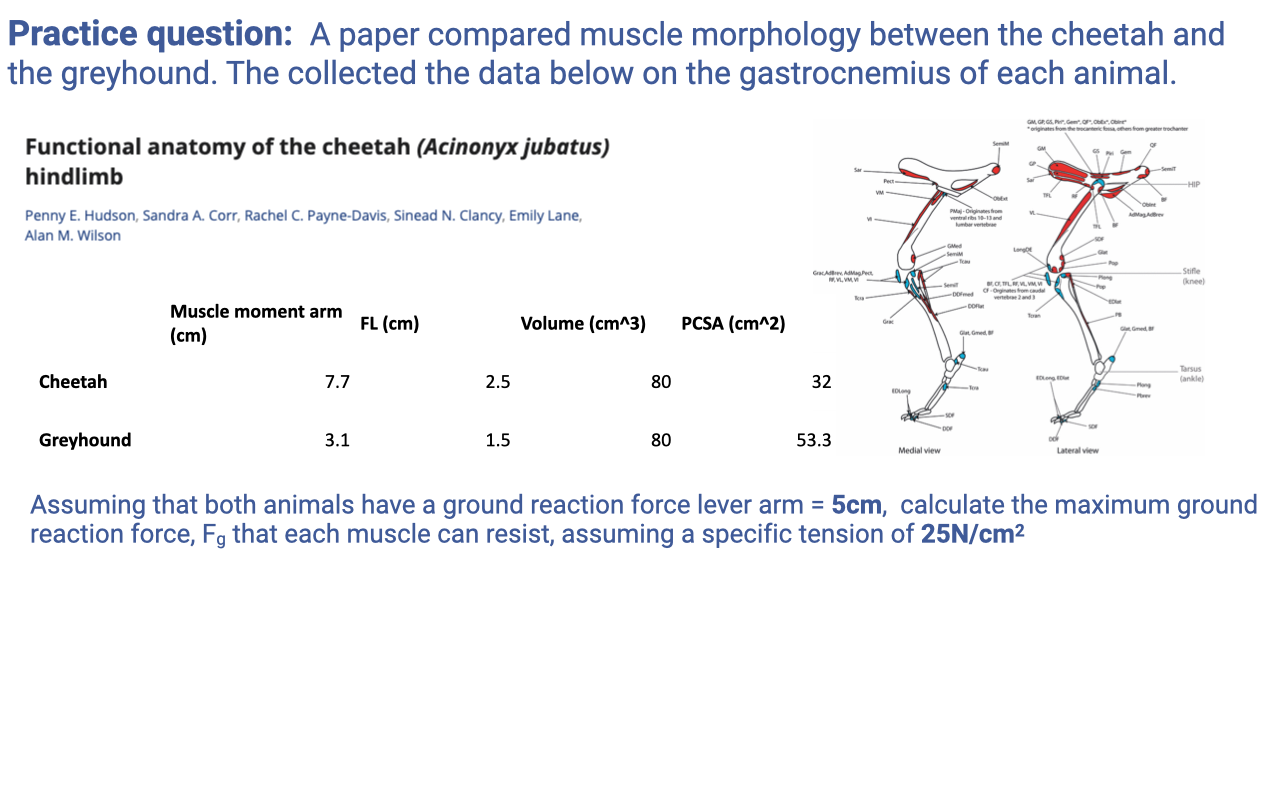
Practice Question 1B — Maximum Ground Reaction Force

Now the table is augmented with PCSA (verifying the Volume/FL calculation from Slide 16):
- Cheetah: 80 / 2.5 = 32 cm²
- Greyhound: 80 / 1.5 ≈ 53.3 cm²
Setup: both animals have a ground reaction force lever arm = R = 5 cm about the ankle (i.e., the distance from the GRF vector to the ankle joint center). Specific tension = 25 N/cm². Find the maximum GRF (F_g) that the muscle can resist.
Step 1 — Maximum muscle force:

\[F_m = \text{PCSA} \times \sigma_{\text{spec}}\]

Cheetah: $F_m = 32 \times 25 = 800$ N
Greyhound: $F_m = 53.3 \times 25 \approx 1333$ N
Step 2 — Lever-system equation (torque balance about the ankle):

\[F_m \cdot r_m = F_g \cdot R\] \[F_g = F_m \cdot \frac{r_m}{R}\]

where $r_m$ = muscle moment arm and $R$ = GRF moment arm = 5 cm.

Step 3 — Solve:
- Cheetah: $F_g = 800 \times \frac{7.7}{5} = 800 \times 1.54 \approx 1232$ N
- Greyhound: $F_g = 1333 \times \frac{3.1}{5} = 1333 \times 0.62 \approx 826$ N
Interpretation:
- Cheetah can resist a larger GRF (~1232 N) at the foot because of its larger muscle moment arm — the lever amplifies the muscle’s force at the ground.
- Greyhound has a higher PCSA and stronger muscle at the tendon, but its smaller moment arm means less of that force translates to a foot-on-ground force.
- Reinforces the EMA concept: the same muscle force can be turned into either higher joint torque (large $r_m$) or higher angular velocity (small $r_m$). The cheetah favors torque; the greyhound favors angular speed.

Slide 18

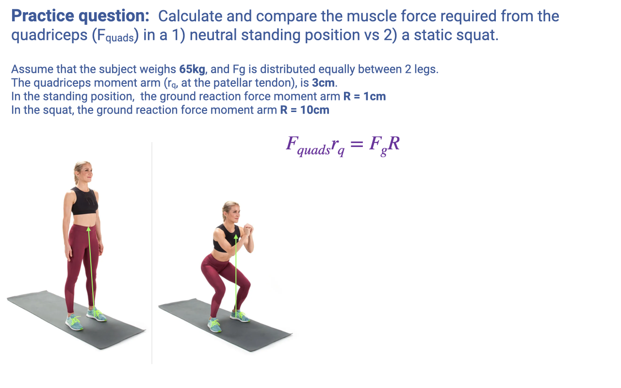
$Slide titled "Practice question: Calculate and compare the muscle force required from the quadriceps (F_quads) in a 1) neutral standing position vs 2) a static squat." Body of the slide: "Assume that the subject weighs 65 kg, and Fg is distributed equally between 2 legs. The quadriceps moment arm (r_q), at the patellar tendon, is 3 cm. In the standing position, the ground reaction force moment arm R = 1 cm. In the squat, the ground reaction force moment arm R = 10 cm." The lever-system equation $F_{quads} \cdot r_q = F_g \cdot R$ is shown in purple. Two photographs at the bottom show a young woman first in a neutral standing position (left) and then in a deep static squat with knees flexed and hips lowered (right), wearing red leggings and a black sports top.$

Practice Question 2 — Quadriceps Force in Standing vs Static Squat

Setup: 65-kg subject, GRF split equally between two legs.
- $F_g$ per leg $= \frac{1}{2} \times 65 \text{ kg} \times 9.81 \text{ m/s}^2 \approx \frac{637.7}{2} \approx 319$ N
Quadriceps moment arm (at the patellar tendon): $r_q = 3$ cm = constant.
GRF moment arm at the knee changes with posture:
- Standing: $R = 1$ cm (GRF passes nearly through the knee — almost no torque).
- Squat: $R = 10$ cm (GRF is well behind the knee — large knee-flexion torque).
Lever-system equation (torque balance about the knee):

\[F_{\text{quads}} \cdot r_q = F_g \cdot R\] \[F_{\text{quads}} = F_g \cdot \frac{R}{r_q}\]

Solve:
- Standing: $F_{\text{quads}} = 319 \times \frac{1}{3} \approx 106$ N
- Squat: $F_{\text{quads}} = 319 \times \frac{10}{3} \approx 1063$ N
The quadriceps must produce ~10× more force in the static squat than standing — purely because of the change in moment-arm ratio. The body weight has not changed at all.
Why this matters:
- Explains why holding a deep squat is fatiguing even with no movement and no added load — the isometric force demand on the quadriceps is large.
- Demonstrates mechanical disadvantage at deep knee flexion: the closer the GRF moves away from the knee, the greater the torque the quadriceps must oppose.
- This is a safety-of-loading lesson too: weight-room exercises that combine deep-squat geometry with added external load can multiply quadriceps tendon forces dramatically — explaining why patellar tendon injuries are common in heavy squatting.
Reinforces the broader Week 6 message: lever geometry matters as much as muscle physiology in determining the force required for a given task.

Slide 19

Practice Question 3 — Sketch the Three Idealized Work Loops

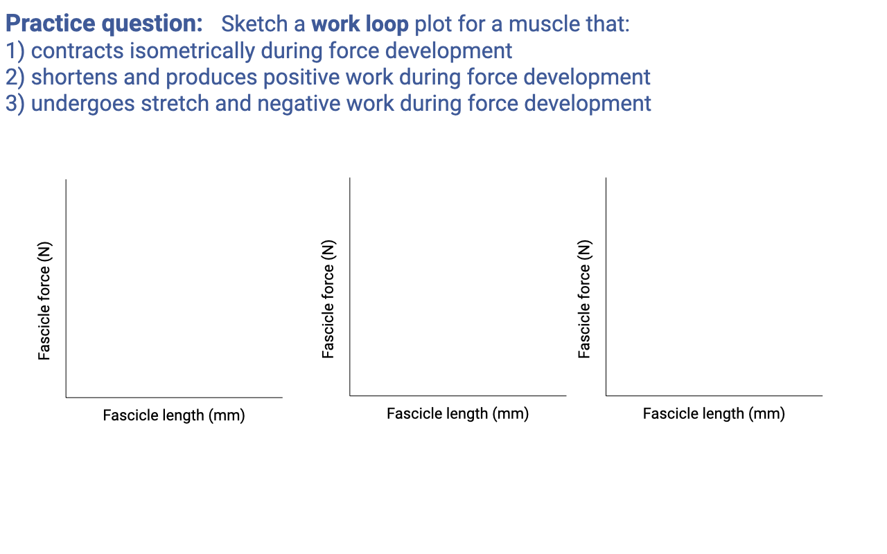
Goal: sketch the work-loop shape (force vs length) for each of three contraction types. The area enclosed = net work done by the muscle; the direction of travel (counterclockwise vs clockwise) determines the sign of that work.
(1) Isometric contraction during force development — like the turkey gastrocnemius during level running (Slide 3, Slide 4):
- Length is nearly constant while force rises and falls.
- The loop collapses to a near-vertical line along the y-axis at a single length.
- Net work ≈ 0 (no displacement → no work, even though force is high).
- Tendon and other series-elastic elements still cycle energy elastically — only the muscle itself does no net work.
(2) Shortening with positive work during force development — like the cockatiel pectoralis or guinea fowl gastrocnemius on an incline (Slide 4):
- As the muscle activates, it shortens while producing high force.
- The loop has a counter-clockwise sense (force-up → shorten-with-high-force → force-down → re-lengthen-passively).
- Net work is positive — the enclosed area opens up in the upper-left of the F–L plane.
- The muscle is acting as a motor, delivering net energy to the system.
(3) Stretch with negative work during force development — like the guinea fowl digital flexor at landing (Slide 4) or any muscle absorbing energy at impact:
- The muscle lengthens while producing high force (forced to elongate by external load).
- The loop has a clockwise sense.
- Net work is negative — the enclosed area lies in the lengthening direction; the muscle absorbs energy from the system (which dissipates as heat or is stored briefly).
- The muscle is acting as a brake or damper.
These three shapes — vertical line, counterclockwise loop, clockwise loop — encode the three fundamental mechanical roles a muscle can play: strut/spring (no net work), motor (positive work), and brake (negative work). Every in vivo muscle work loop in this lecture (turkey, wallaby, cockatiel, guinea fowl, mallard, Lai et al. soleus) is a real-world variation on one of these three idealized templates.

Key Equations

Equation	Name	Description
$F_m = \text{PCSA} \times \sigma_{\text{spec}}$	Maximum isometric muscle force	Maximum force a muscle can produce equals its physiological cross-sectional area times specific tension (~20–30 N/cm²). PCSA = muscle volume / fiber length.
$F_m \cdot r_m = F_g \cdot R$	Lever-system equation (torque balance)	Muscle force × muscle moment arm = external force × external moment arm. Used in the cheetah/greyhound and squat practice problems to convert between muscle force and ground reaction force.
$\text{EMA} = r_m / R$	Effective mechanical advantage	Ratio of muscle moment arm to ground-reaction-force moment arm at a joint. High EMA → less muscle force needed to resist a given GRF; varies systematically with body size and posture.
$W = \oint F \, dL$	Work loop (net mechanical work)	Net work done by a muscle equals the area enclosed by its force–length trajectory over a contraction cycle. Sign depends on direction of travel: counterclockwise = positive (motor), clockwise = negative (brake), no enclosed area = strut/spring.
$\text{Power} = F \times V$	Mechanical power	Power output of a muscle is force times shortening velocity; for cyclic contractions, mean power = (net work per cycle) × (cycle frequency).

Glossary of Key Terms

Term	Definition
Inverse dynamics	Indirect method that uses measured kinematics and ground reaction forces to compute the net joint torque and joint work at each joint. Cannot resolve individual-muscle behavior because multiple muscles cross every joint and the tendon can decouple muscle and joint motion.
Sonomicrometry	Direct method using small piezoelectric crystals implanted in muscle to measure fascicle length dynamically; combined with a tendon force buckle to record muscle force. The technique used by Roberts et al. (1997) in turkeys.
B-mode ultrasound	Non-invasive imaging technique that resolves fascicle length and pennation angle in real time in living humans during walking, running, or cycling; the human analog of sonomicrometry.
Muscle work loop	Plot of muscle force vs. muscle length over a single contraction cycle. The enclosed area equals net mechanical work; the direction of travel sets the sign. Standard graphical tool for classifying muscle function as motor, spring/strut, or brake in vivo.
Strut (in muscle function)	A muscle that contracts near-isometrically during force development, allowing the tendon to act as a passive spring. Produces no net muscle work but is essential for transmitting force to the skeleton.
Motor (muscle function)	A muscle that shortens while producing high force, generating substantial positive net work. Specialized motors include cockatiel pectoralis and mallard gastrocnemius.
Brake / energy absorber	A muscle that lengthens while producing high force, doing negative net work — dissipating energy from the system. Often seen in distal limb muscles at heel-strike (e.g., guinea fowl digital flexor).
Multifunctional muscle	A muscle whose architecture allows it to act as a strut on level ground and a motor on inclines or during acceleration. Turkey lateral gastrocnemius is the canonical example.
Spring specialist	A muscle with extreme architecture (very short fibers, very long thin tendon) that is constrained to act primarily as part of an elastic spring — wallaby plantaris, ostrich/horse distal limb muscles. Trade-off: low safety factor for tendon injury.
Generalist muscle	A muscle of intermediate architecture that does modest positive work in steady gait, can upregulate for inclines, and provides stability on uneven terrain (e.g., guinea fowl gastrocnemius).
Proximo-distal gradient	The pattern in cursorial limbs of placing high-mass power-producing muscles proximally (hip, shoulder) and specialized short-fibered muscles with long tendons distally (ankle, wrist). Reduces distal-limb inertia and allows elastic energy cycling.
Plantigrade vs digitigrade vs unguligrade posture	Three foot postures along a continuum of distal-limb elongation. Plantigrade (humans, bears) — flat foot on ground; digitigrade (dogs, cats, birds) — toes on ground, foot bones elongated as a third leg segment; unguligrade (horses, ungulates) — only the tips of the toes on ground, maximal distal-limb elongation.
Effective mechanical advantage (EMA)	$r_m/R$ — the ratio of muscle moment arm to ground-reaction-force moment arm at a joint. Cheetah gastrocnemius (slide 17) has higher EMA than greyhound; large mammals have higher EMA than small mammals (Biewener scaling, Lecture 13).
Specific tension ($\sigma_{\text{spec}}$)	Maximum isometric force per unit cross-sectional area of muscle, ~20–30 N/cm² (often 25 N/cm² as in the practice problem). Sets the conversion from PCSA to maximum muscle force.
Walk-to-run gait transition	The speed at which humans (and other bipeds) switch from walking to running. Lai et al. (2015) showed the transition keeps the soleus closer to its optimal F–L and F–V operating point — a metabolic and mechanical optimum.
Ankle exoskeleton (passive)	A wearable device with a rotational spring in series with the Achilles tendon that stores and returns energy during stance. Effective only when its stiffness is tuned to the muscle-tendon unit it augments — too stiff and metabolic cost rises; too compliant and there is no benefit.
Running blade prosthesis	A passive carbon-fiber lower-limb prosthesis designed as an elastic spring that mimics the Achilles-tendon stretch-recoil function during running. Stiffness must be individualized; no single optimal stiffness exists across athletes (Taboga et al. 2020).
Godoy Fellowship	Dr. M. Marlene Godoy Fellowship in Movement Sciences — a UCI CIMS-administered summer research fellowship offering $4,000 over 10 weeks for undergraduates working with a CIMS-affiliated faculty sponsor. Application linked from cims.uci.edu.