Lecture 12: Introduction to Muscle Structure and Function 2 — Tissue Scale

Slide 1

• Continues the muscle physiology section from Lecture 11, building from the cellular scale up to the tissue scale of muscle function.
• Today’s focus: the intrinsic mechanical properties of muscle as a tissue — the force-length and force-velocity relationships and how they translate molecular cross-bridge dynamics into whole-muscle behavior.
• A central message: muscle’s intrinsic properties produce a trade-off between force and displacement at the molecular and tissue level, and different optimal contraction conditions maximize force, speed, power, or efficiency.

---

Slide 2

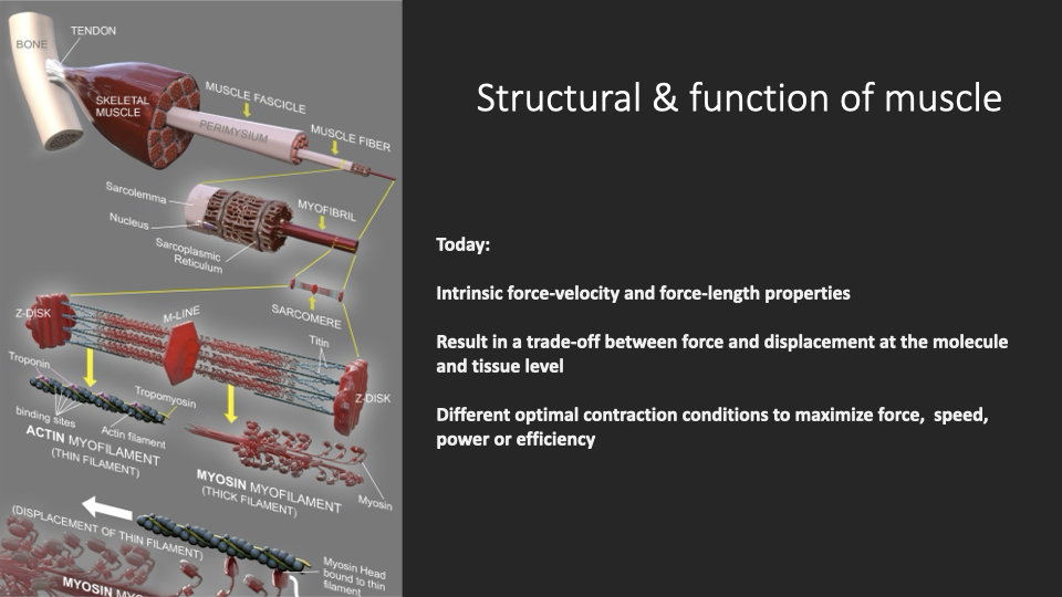
Today: From Molecules to Tissue Properties

• Tissue-scale intrinsic properties of muscle:
  • Force–length (length–tension) relationship.
  • Force–velocity relationship.
• These properties emerge from the molecular machinery (sliding filaments, cross-bridge cycling) but operate at a different scale of analysis.
• They formalize a trade-off between force and displacement that runs from the molecular level (overlap of actin and myosin) all the way to whole-tissue mechanics.
• Different points on these curves yield optimal conditions for force, speed, power, or efficiency — no single muscle state can maximize all of them simultaneously.

---

Slide 3

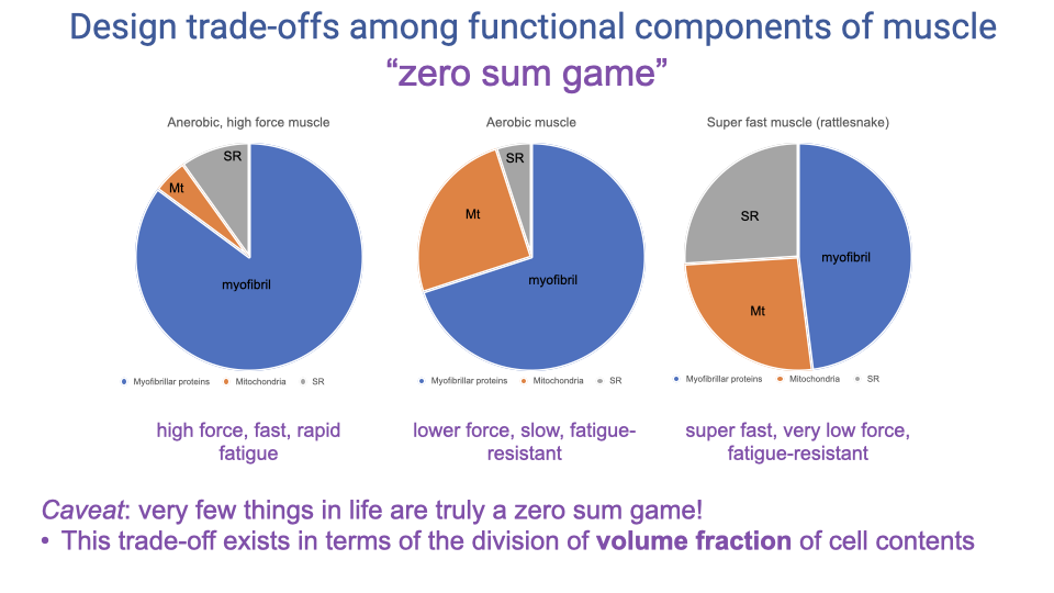
Recap — The “Zero-Sum Game” of Muscle Volume Fractions

• Recap from Lecture 11: a fixed muscle-cell volume must be partitioned among myofibrils (force), SR (activation/relaxation speed), and mitochondria (aerobic ATP).
• The three example pie charts (anaerobic high-force, aerobic, super-fast rattlesnake) each represent different solutions on the trade-off surface.
• The zero-sum game describes the division of volume fraction in a fixed cell; it is not an absolute trade-off in capacity.

---

Slide 4

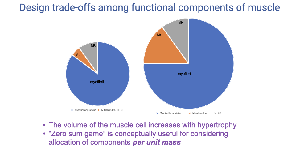
Hypertrophy Breaks the Strict Zero-Sum Game

• With training, the volume of the muscle cell increases (hypertrophy) — so absolute amounts of all three components can grow simultaneously.
• The zero-sum game still applies in per-unit-mass terms (you can’t have a high mass-specific everything), but it does not apply in absolute terms.
• Why this matters: carrying mass is energetically costly, so animals trade off mass-specific capacity (proportions) against absolute capacity (whole-muscle mass).

---

Slide 5

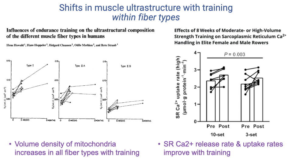
Within-Fiber-Type Plasticity (Recap)

• Both mitochondrial volume density and SR Ca²⁺-handling rates improve with training within each fiber type, not just by shifting fiber-type proportions.
• This further illustrates that fiber type is a continuum, not a strict category, and that the cellular components are individually plastic.
• Together with hypertrophy, these adaptations explain why elite athletes can achieve combinations of force, speed, and endurance that look like violations of the zero-sum game.

---

Slide 6

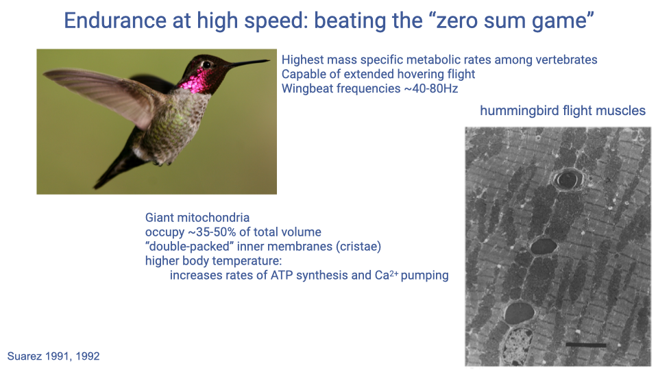
Hummingbirds Push the Trade-off Surface

• Hummingbirds combine extreme aerobic capacity with high contraction frequency:
  • Highest mass-specific metabolic rates of any vertebrates.
  • Hovering flight sustained for prolonged periods.
  • Wingbeat frequencies of ~40–80 Hz.
• Their flight muscles have:
  • Giant mitochondria occupying ~35–50% of cell volume (well beyond typical vertebrate muscle).
  • Double-packed cristae (extra inner membrane).
  • Operating temperatures elevated above typical body temperature, accelerating ATP synthesis and Ca²⁺ pumping.
• These specializations expand the cellular envelope rather than violating the zero-sum trade-off.

---

Slide 7

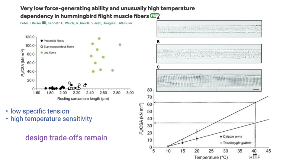
Hummingbird Trade-offs — Low Specific Tension and Thermal Sensitivity

• The “broken zero-sum game” of hummingbird flight muscle comes with its own costs:
  • Very low specific tension (force per unit cross-sectional area) — because so much volume is mitochondria, less is myofibrils.
  • High temperature sensitivity — force falls off steeply at lower temperatures.
• Functional consequence: hummingbirds enter torpor in cold conditions because muscle force collapses below their narrow operating temperature range.
• Design trade-offs remain — even extreme specialists pay for one capacity with another.

---

Slide 8

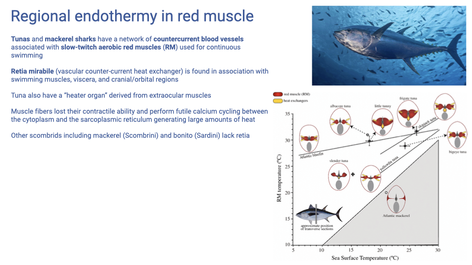
Regional Endothermy and Heater Organs

• Tunas and mackerel sharks maintain elevated red-muscle temperature above ambient water using a rete mirabile — a vascular countercurrent heat exchanger that traps metabolic heat near the slow-twitch aerobic red muscle used for continuous swimming.
• The rete also occurs in association with viscera and cranial/orbital regions in some species.
• Heater organs: in some tunas, extraocular muscles have lost contractile function and instead perform futile Ca²⁺ cycling between cytoplasm and SR — generating heat to warm the eye and brain.
• Other scombrids (mackerel, bonito) lack retia, so this is a derived feature within the group.
• Reinforces the importance of muscle temperature for muscle function — and shows that the molecular machinery of muscle can be co-opted for thermogenesis when the contractile function is lost over evolutionary time.

---

Slide 9

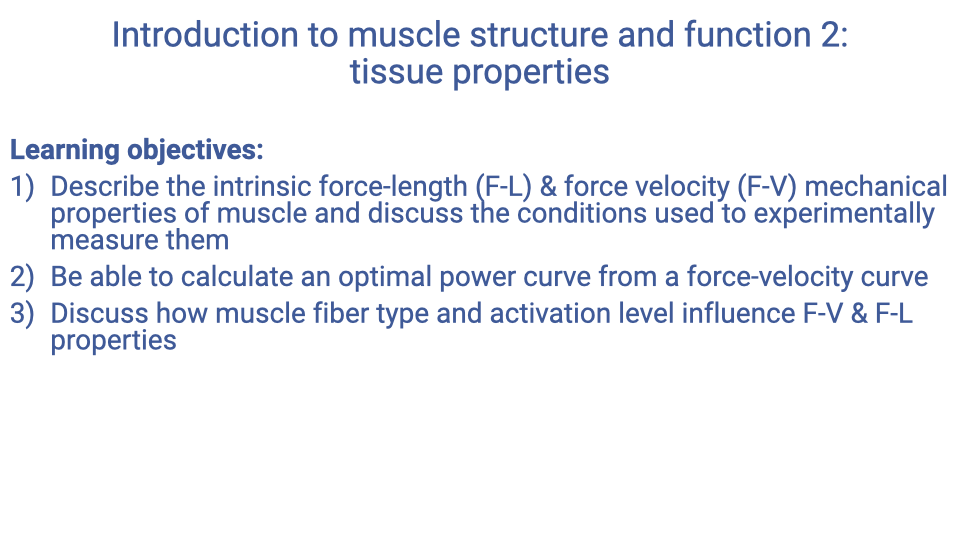
Learning Objectives — Tissue Properties

1. Describe the intrinsic force–length (F–L) and force–velocity (F–V) mechanical properties of muscle and discuss the experimental conditions used to measure them.
2. Be able to calculate an optimal power curve from a force–velocity curve.
3. Discuss how muscle fiber type and activation level influence F–V and F–L properties.

---

Slide 10

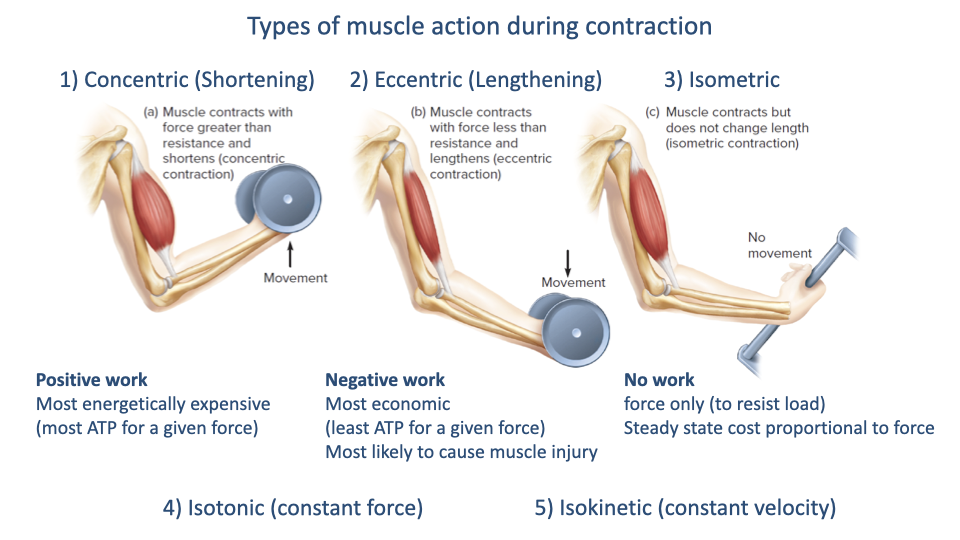
Types of Muscle Action — Concentric, Eccentric, Isometric, Isotonic, Isokinetic

Action	Description	Energetic cost
Concentric (shortening)	Muscle force > load; muscle shortens; positive work	Most expensive ATP per unit force
Eccentric (lengthening)	Muscle force < load; muscle lengthens; negative work	Most economic; highest injury risk
Isometric	Force generated, no length change; no work	Steady-state cost proportional to force
Isotonic	Constant force during shortening; experimental condition	—
Isokinetic	Constant velocity during shortening; experimental condition	—

• These action types matter physiologically: e.g., you can jump down from a higher height than you can jump up to — eccentric contractions produce higher force, more economically, than concentric contractions.
• Isotonic and isokinetic are mainly laboratory conditions used to isolate one variable (force or velocity) — they map onto the F–V experiments below.
• Isometric work with elastic tendon stretch–recoil is common in locomotion (e.g., running) and is economical because the muscle does no shortening work.

---

Slide 11

The Two Intrinsic Curves

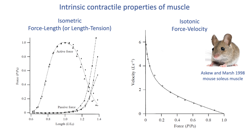
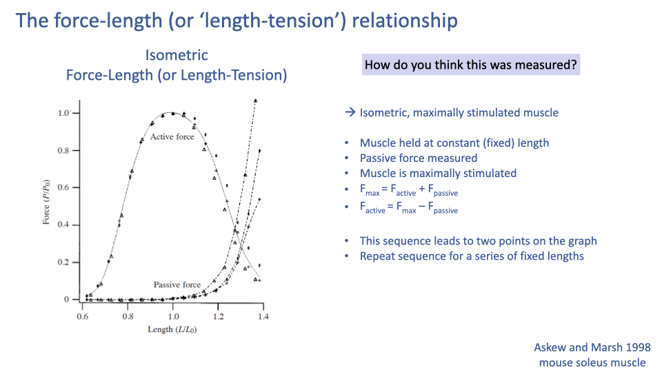
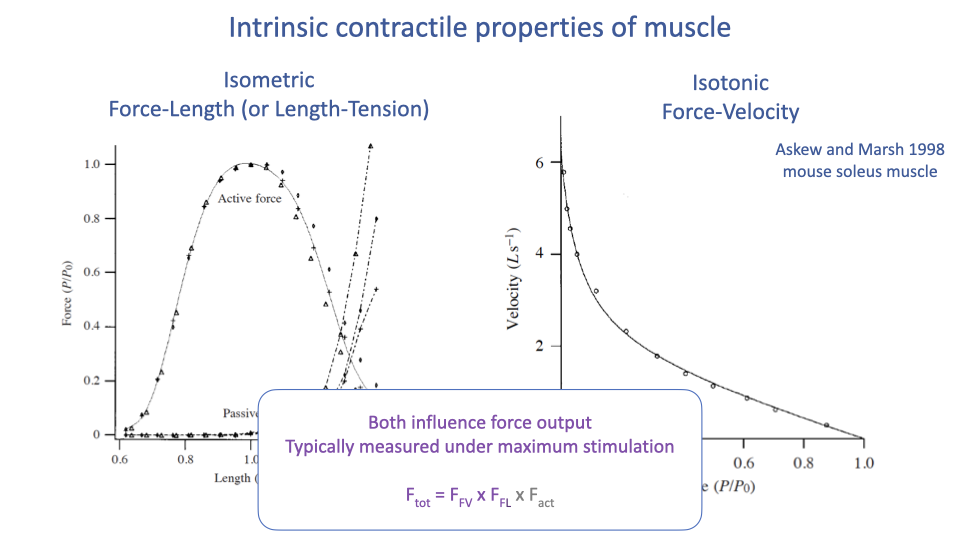
• Isometric force–length (length–tension): the maximum active force a muscle can produce as a function of its length.
  • Parabolic shape with a peak at the optimum length L₀.
  • Passive force (from connective tissue and titin) rises exponentially at long lengths.
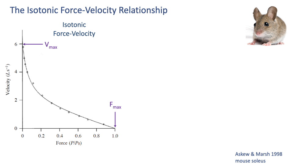
• Isotonic force–velocity: the maximum shortening velocity a muscle can sustain at a given constant force.
  • Hyperbolic shape (Hill-type curve).
  • V_max at zero force; F_max at zero velocity.
• These two curves are the foundation of all muscle modeling — including the musculoskeletal simulations used in clinical biomechanics (e.g., OpenSim).

---

Slide 12

Mechanism of the Length–Tension Curve at the Sarcomere Level

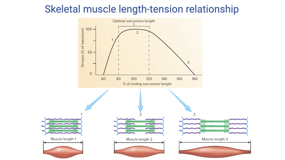
• The active force–length curve is mechanistically explained by actin–myosin filament overlap:
  • Short lengths: actin filaments cross past each other and myosin filaments butt against the Z-discs → interference and reduced cross-bridge formation.
  • Optimal length (~100% of resting sarcomere length, plateau ~80–120%): maximal overlap of actin binding sites with myosin heads → maximum cross-bridge formation.
  • Long lengths: filament overlap decreases → fewer cross-bridges can form → force falls.
• The plateau region in whole-muscle data exists because individual sarcomeres in a muscle are not all at exactly the same length — the variation smears out the sharp peak predicted at the single-sarcomere level.

---

Slide 13

Setup — How Was the F–L Curve Measured?

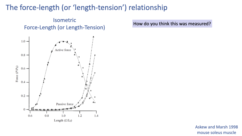
• The slide poses the measurement question: how was this curve actually generated experimentally?
• Important conceptual point: the curve is not measured by stretching one muscle while it contracts.
• Each point is generated under strict isometric, maximally stimulated conditions at a series of different fixed lengths (next slide).

---

Slide 14

How the F–L Curve Is Measured (Protocol)

1. Mount the muscle (or fiber) in a muscle ergometer — a rig that fixes the muscle at a given length while measuring force.
2. Hold the muscle at a constant length; measure the passive force at that length (no stimulation).
3. Maximally stimulate the muscle (electrically for a whole muscle, by Ca²⁺-bath for a skinned fiber).
4. Measure the maximum force during isometric contraction at that length: $F_{max} = F_{active} + F_{passive}$.
5. Compute: $F_{active} = F_{max} - F_{passive}$.
6. Repeat at a series of fixed lengths; each length yields one passive point and one active point on the curve.

• There is no single experiment in which a muscle continuously sweeps through this curve. The F–L curve is assembled from many independent isometric trials — it is an “envelope” of maximum capability, not a record of any single contraction.

---

Slide 15

Real Data — Guinea Fowl Lateral Gastrocnemius

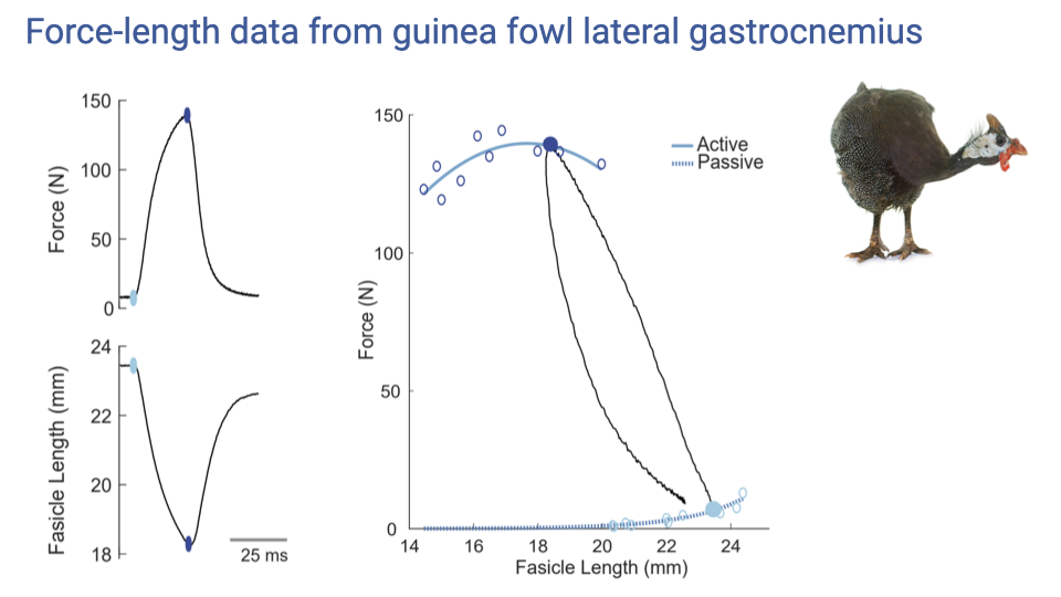
• An example of an actual F–L measurement on the guinea fowl lateral gastrocnemius (a whole muscle–tendon unit).
• During each isometric trial, the fascicles shorten slightly even though the whole muscle–tendon length is fixed — the shortening is taken up by tendon stretch.
• The investigator must wait for the fascicle length to reach steady state before recording the force value; that pair of (fascicle length, force) becomes one point on the F–L curve.
• Repeated trials at many starting lengths fill out the active and passive force–length curves.

---

Slide 16

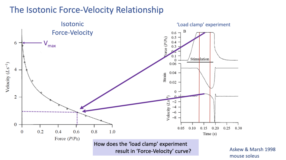
The Isotonic F–V Curve — Endpoints

• V_max: the maximum unloaded shortening velocity (force = 0).
• F_max (also written P₀ or F₀): the maximum isometric force (velocity = 0).
• The shape between these endpoints is hyperbolic — a key intrinsic property of muscle (Hill 1938).

---

Slide 17

How the F–V Curve Is Measured — The Load Clamp

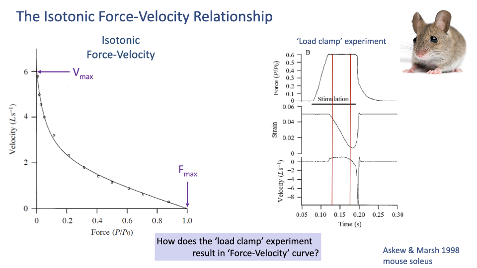
• The load clamp experiment holds the muscle force at a specified constant value while letting it shorten.
• Procedure:
  1. Stimulate the muscle.
  2. As force rises, clamp it at a target value (e.g., 0.6 × F_max).
  3. Once the target force is reached, allow the muscle to shorten freely while maintaining the clamped force.
  4. Measure the steady-state shortening velocity during the clamp.
• That velocity, paired with the clamped force, becomes one point on the F–V curve.

---

Slide 18

Mapping a Load-Clamp Trial to the F–V Curve

• The diagram shows how the clamped force (top panel of the inset, ~0.6 P/P₀) and the steady-state shortening velocity (bottom panel, ~1 L s⁻¹) are read off and mapped to a single point on the F–V curve.
• Repeating the experiment at many different clamp forces generates the full curve.
• This is again an envelope — each point is from a separate, controlled trial.

---

Slide 19

Real Data — Guinea Fowl F–V Curve

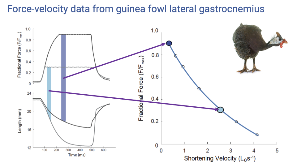
• Two example load-clamp trials on the guinea fowl lateral gastrocnemius:
  • High clamp force (~0.9 F_max) → slow shortening (low velocity point).
  • Lower clamp force (~0.3 F_max) → fast shortening (high velocity point).
• Repeating at many force levels yields the full F–V hyperbola for that muscle.
• Why force and velocity trade off (cross-bridge mechanism): at higher shortening velocities, more myosin heads are detached at any moment because they spend more time cycling; at zero velocity (isometric), all cross-bridges can be simultaneously attached, giving maximum force.

---

Slide 20

Body Size and V_max — Small Animals Have Faster Muscles

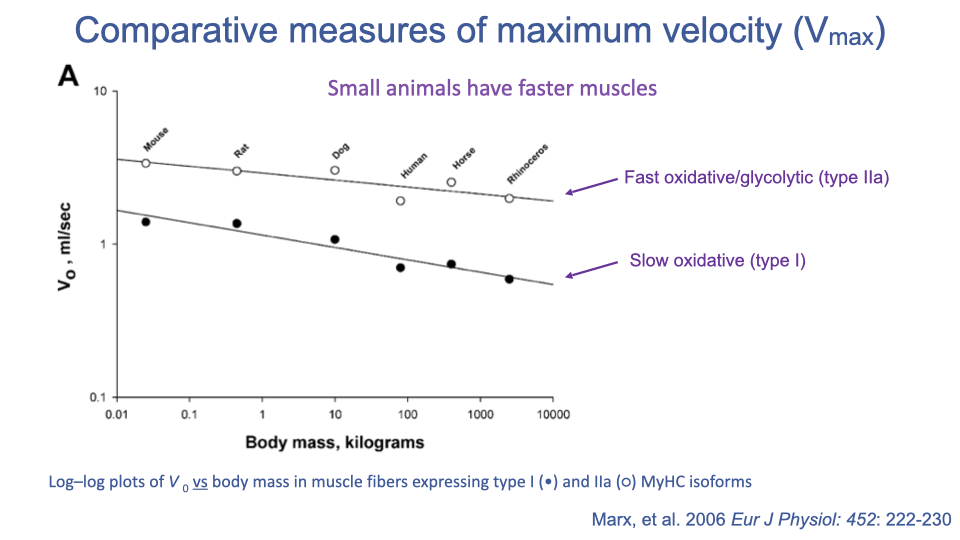
• Across mammals, both type I and type IIa fibers show decreasing V_max with increasing body mass.
• Functional rationale: larger animals take longer, slower strides to cover a given distance, so the selective pressure for fast muscles is weaker; meanwhile, fast muscles are energetically expensive.
• Fiber type offset: type IIa (fast) > type I (slow) at every body size.

---

Slide 21

Body Size and Maximum Power — With Caveats

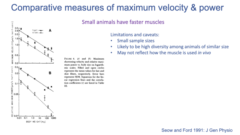
• Both maximum velocity and relative maximum power decrease with body size in mass-specific terms.
• Caveats:
  • Small sample sizes in comparative studies.
  • High within-size diversity — muscle is highly plastic and varies among muscles within an organism.
  • Lab measurements may not reflect in vivo use: animals of different sizes have different mechanical demands and use their muscles differently.

---

Slide 22

Combining F–V, F–L, and Activation

• Both intrinsic curves are typically measured at maximum stimulation — they describe the upper envelope of force capability.
• A widely used muscle model combines them multiplicatively:

\[F\_{tot} = F\_{FV} \times F\_{FL} \times F\_{act}\]

• Where:
  • F_FV: scaling factor from the force–velocity curve at the current shortening velocity.
  • F_FL: scaling factor from the force–length curve at the current length.
  • F_act: activation level (between 0 and 1).
• Used in clinical and research musculoskeletal models (e.g., OpenSim) to predict how muscles will perform under different movements and surgical interventions (e.g., tendon transfers, shoulder reconstruction).

---

Slide 23

The 3D Force–Length–Velocity Surface

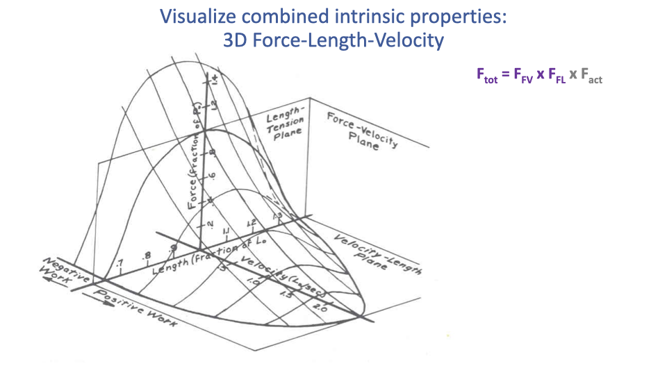
• At maximum activation, the muscle’s force capability is fully described by a 3D surface: the product of the F–L parabola and the F–V hyperbola.
• This surface defines the action space of the muscle:
  • Highest force at optimal length and zero velocity.
  • Force falls off away from optimal length (in either direction).
  • Force falls off with increasing shortening velocity.
• Any in vivo contraction corresponds to a trajectory across this surface; the resulting force is read off the surface at the current length and velocity.

---

Slide 24

Activation Level Scales the F–V Curve

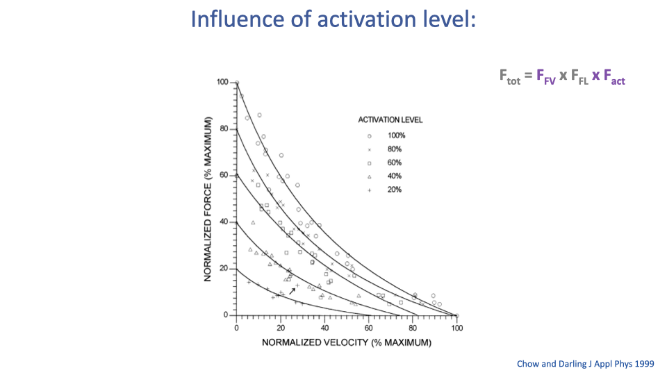
• A hyperbolic F–V relationship exists at every activation level, not just at 100%.
• Lower activation produces a lower-amplitude curve — both maximum force and maximum velocity decrease.
• In standard muscle models, activation is often assumed to scale the entire surface proportionally (multiplicatively) — though there is now growing evidence that the curve shape changes at submaximal activation as well (see Slide 28).

---

Slide 25

Activation in 3D — Nesting Surfaces

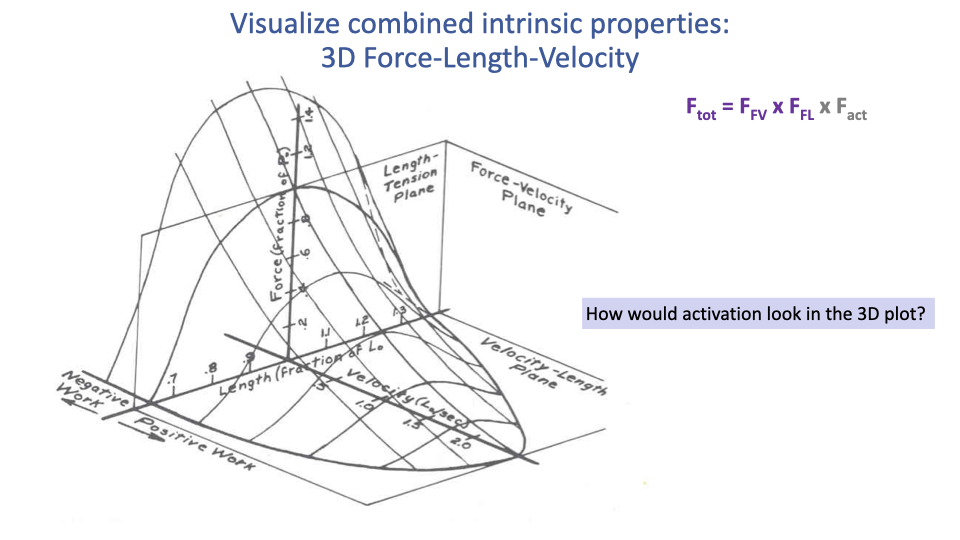
• Conceptually, lower activation corresponds to a smaller, nested 3D surface stacked beneath the maximally activated surface.
• An apt metaphor: Russian nesting dolls — each activation level produces a similarly shaped but smaller F–L–V surface.
• The full muscle model therefore lives in a 4D space (force × length × velocity × activation).

---

Slide 26

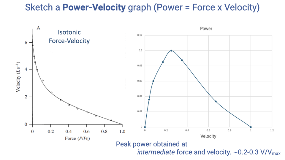
Constructing the Power–Velocity Curve

• Power = Force × Velocity at every point on the F–V curve.
• Power is zero at the endpoints (zero velocity → zero displacement → no power; zero force → no work done) and reaches a single peak at intermediate force and velocity.
• Peak power typically occurs at roughly 0.2–0.3 × V_max for vertebrate skeletal muscle.
• There is an optimal contraction velocity for power output — for example, this is why bicycles need gears, so cyclists can keep their muscles operating near their optimal cadence regardless of road speed or grade.

---

Slide 27

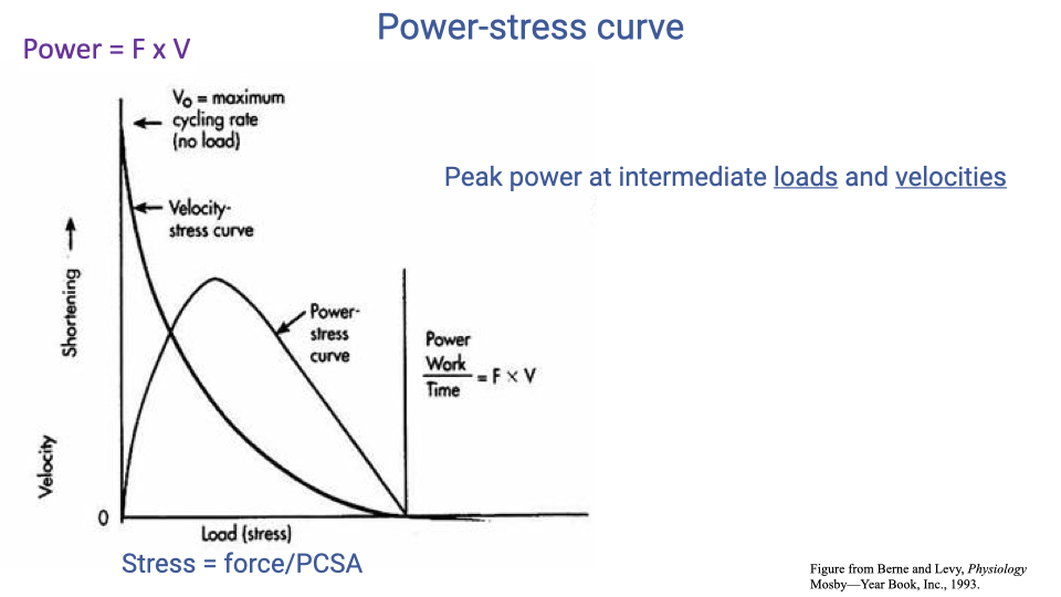
Power–Stress Curve and Cross-Sectional Normalization

• An equivalent way to plot the same relationship: power vs. load (stress) instead of power vs. velocity.
• Stress = force per physiological cross-sectional area (PCSA) — normalizes for muscle size.
• Same general result: peak power at intermediate loads and velocities.
• The shape of these curves is foundational for understanding why athletes train at specific resistance levels and why muscle architecture (PCSA, fiber length) matters for whole-muscle power output.

---

Slide 28

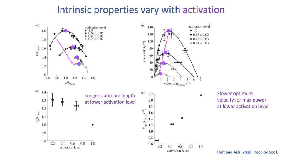
The Curves Themselves Change With Activation

• New experimental evidence (Holt and Azizi 2016): the F–L and F–V curves change shape — not just amplitude — with activation level.
• Key effects at lower activation:
  • Optimum length L₀ shifts to longer fiber lengths.
  • Optimum velocity for peak power V_opt shifts to slower velocities.
• Implication for muscle modeling: the simple multiplicative model ($F_{tot} = F_{FV} \times F_{FL} \times F_{act}$) is an approximation — at submaximal activation (which is typical of most everyday movements!), more sophisticated models are required.

---

Slide 29

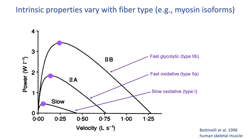
F–V and Power Vary With Fiber Type

• Different myosin isoforms produce different F–V hyperbolas — and therefore different power curves.
• In human skeletal muscle (Bottinelli et al. 1996):
  • Type IIB (fast glycolytic): highest V_max and highest peak power, at the highest optimum velocity.
  • Type IIA (fast oxidative): intermediate.
  • Type I (slow oxidative): lowest V_max, lowest peak power, slowest optimum velocity.
• All three curves share the same fundamental hyperbolic shape, but their scale and curvature differ.
• These differences are why fiber type composition of a muscle matters so much for sport-specific performance.

---

Slide 30

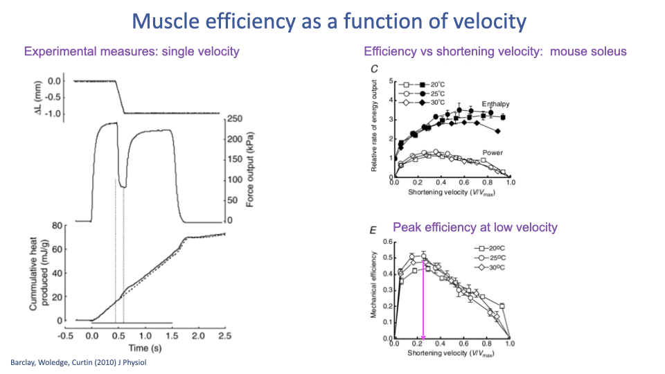
Efficiency Peaks at Low Velocity

• Mechanical efficiency (work output ÷ total energy expenditure) is a function of shortening velocity.
• Across temperatures (20–30°C in mouse soleus), efficiency:
  • Peaks at low shortening velocity (~0.1–0.2 V/V_max).
  • Falls off at higher velocities as more energy is lost as heat.
• The velocity that maximizes power (~0.25 V/V_max) is higher than the velocity that maximizes efficiency — animals (and athletes) face a trade-off between going fast and using fuel efficiently.

---

Slide 31

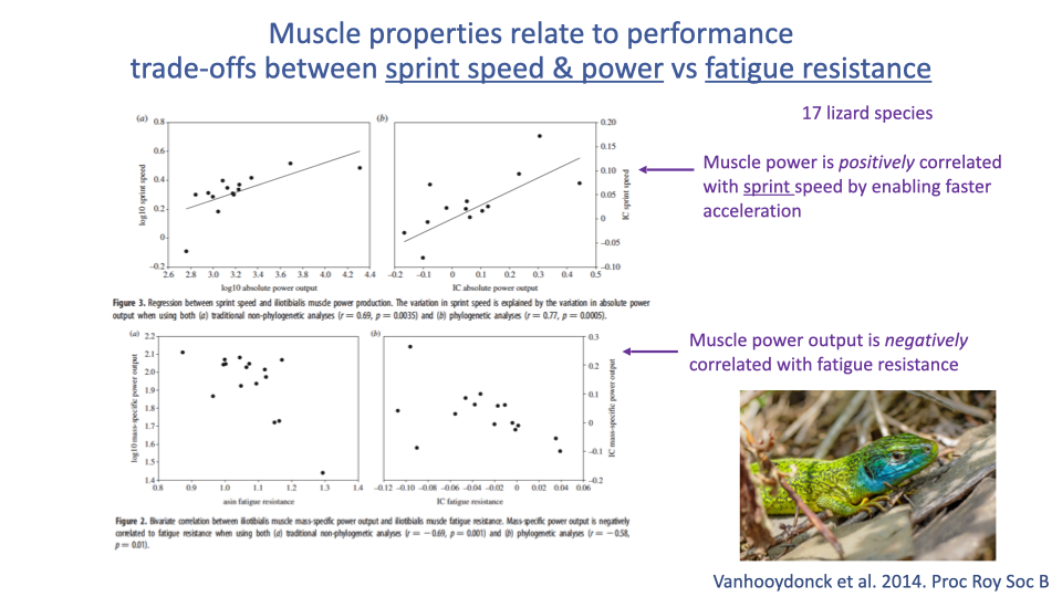
Sprint Power vs. Fatigue Resistance — A Comparative Trade-off

• Across 17 lizard species (Vanhooydonck et al. 2014):
  • Mass-specific muscle power is positively correlated with sprint speed (high power → fast acceleration).
  • Mass-specific muscle power is negatively correlated with fatigue resistance.
• This is the whole-organism manifestation of the cellular zero-sum game from Lecture 11: species that have evolved high sprint power have done so at the cost of endurance.
• A clean comparative example of how intrinsic muscle properties translate into ecological performance trade-offs.

---

Slide 32

Learning Objectives — Recap

1. Intrinsic F–L and F–V properties: assembled from many isometric (F–L) or isotonic load-clamp (F–V) trials, each at maximum stimulation; they form envelopes, not records of single contractions.
2. Power from F–V: power = force × velocity, so the power–velocity curve is computed point-by-point from the F–V curve. Peak power occurs at intermediate force and velocity (~0.2–0.3 V_max).
3. Fiber type and activation effects: faster fiber types have higher V_max and higher peak power; activation scales the F–V/F–L surface and (per recent work) also shifts its optimal length and velocity.

---

Key Equations

Equation	Name	Description
$F_{max} = F_{active} + F_{passive}$	Total isometric force	Measured force during maximally stimulated isometric contraction is the sum of active (cross-bridge) force and passive (titin + connective tissue) force.
$F_{active} = F_{max} - F_{passive}$	Active force	Active force is computed by subtracting separately measured passive force from the total. Used to construct the active F–L curve point-by-point.
$(V + b)(F + a) = b(F_0 + a)$	Hill force–velocity equation	The classic hyperbolic relation between shortening velocity $V$ and load $F$. $F_0$ is the maximum isometric tension (at $V = 0$); $V_0$ is the maximum shortening velocity (at $F = 0$); $a$ is a coefficient related to the heat of shortening; $b = a(V_0/F_0)$.
$P = F \cdot V$	Mechanical power	Instantaneous power output; computed point-by-point from the F–V curve. Peak power occurs at intermediate force and velocity (~0.2–0.3 Vmax).
$F_{tot} = F_{FV} \cdot F_{FL} \cdot F_{act}$	Combined muscle model	The standard multiplicative muscle model used in musculoskeletal simulations (e.g., OpenSim): total force is the product of velocity-, length-, and activation-dependent factors.
$\sigma = F / \text{PCSA}$	Specific tension (stress)	Force normalized by physiological cross-sectional area; allows comparison of intrinsic capability across muscles of different sizes.

---

Glossary of Key Terms

Term	Definition
Hypertrophy	Increase in muscle cell volume in response to training; allows simultaneous increases in absolute amounts of myofibrils, mitochondria, and SR even though their fractional volumes still trade off.
Hovering flight	Sustained flight in place; aerodynamically demands lift on both upstroke and downstroke, requiring extreme power output (e.g., hummingbirds).
Pectoralis	Avian downstroke flight muscle; in hummingbirds, exclusively type IIa fibers packed with giant mitochondria.
Supracoracoideus	Avian upstroke flight muscle; routes through a tendon over the shoulder to lift the wing.
Specific tension (P/CSA)	Force generated per unit cross-sectional area; reflects myofibrillar volume fraction and is much lower in hummingbird flight muscle than in standard vertebrate muscle.
Regional endothermy	Maintenance of elevated temperature in selected tissues using vascular countercurrent heat exchangers (e.g., red swimming muscle in tunas).
Rete mirabile	The vascular countercurrent heat exchanger that traps metabolic heat in tissues such as red muscle of tunas and mackerel sharks.
Heater organ	A muscle (e.g., extraocular in some tunas) that has lost contractile function and dedicates its calcium-cycling machinery to thermogenesis via futile Ca2+ cycling.
Concentric contraction	Shortening contraction in which muscle force exceeds the load; performs positive work; most expensive in ATP per unit force.
Eccentric contraction	Lengthening contraction in which the load exceeds muscle force; performs negative work; most economic per unit force; greatest injury risk because sarcomeres can be stretched past overlap.
Isometric contraction	Constant-length contraction with force generation but no shortening; no mechanical work, but ATP cost is proportional to force.
Isotonic contraction	Contraction at constant force; an experimental condition used to isolate the F–V relationship via load clamps.
Isokinetic contraction	Contraction at constant velocity; produced experimentally by an isokinetic dynamometer (also a clinical biomechanics device).
Force–length (length–tension) relationship	The intrinsic relationship between muscle length and the maximum active isometric force it can produce; parabolic with a peak at the optimum length L0, mechanistically explained by actin–myosin filament overlap.
Optimum length (L0)	The fiber/muscle length at which active isometric force is maximum; corresponds to maximal actin–myosin overlap.
Passive force	Force borne by titin and connective tissue at long lengths, independent of activation; measured before stimulation in F–L experiments.
Active force	The Ca2+-dependent, cross-bridge-driven force; computed as Fmax − Fpassive in F–L experiments.
Force–velocity (F–V) relationship	The intrinsic hyperbolic relationship between shortening velocity and load; foundational result of Hill (1938).
Vmax	Maximum unloaded shortening velocity of a muscle fiber; primarily determined by myosin isoform; declines with body size across mammals.
Fmax (P0)	Maximum isometric force at zero velocity.
Load clamp experiment	A muscle ergometer protocol that holds the muscle force at a specified value while measuring the resulting steady-state shortening velocity; used to construct the F–V curve point-by-point.
Muscle ergometer	A laboratory device that controls and measures muscle length and force; the workhorse of in vitro muscle mechanics.
Power–velocity curve	The product of force and velocity computed across the F–V curve; rises from zero, peaks at intermediate velocity (~0.2–0.3 Vmax), and falls to zero at Vmax.
Mechanical efficiency	Mechanical work output divided by total energy expenditure; peaks at lower velocities than peak power, reflecting the cost of cross-bridge cycling at high speeds.
Activation level (Fact)	A scalar (0–1) representing the fraction of fibers active or the level of Ca2+ activation; in standard muscle models scales the F–L–V surface multiplicatively.
3D F–L–V surface	The combined intrinsic action space of a muscle at maximum activation; the product of the F–L parabola and the F–V hyperbola.
OpenSim	Open-source musculoskeletal simulation software widely used for predicting in vivo muscle force from joint motion using F–L, F–V, and activation models.
Physiological cross-sectional area (PCSA)	The cross-sectional area of a muscle measured perpendicular to its fibers; sets the muscle’s maximum force capacity (proportional to number of sarcomeres in parallel).
Sarcomeres in series vs. in parallel	Architectural arrangement that determines, respectively, the muscle’s range of shortening (series) and maximum force (parallel); training type can shift this balance.
Hill-type muscle model	A standard phenomenological muscle model based on the Hill F–V hyperbola, often combined with an F–L curve and an activation factor.