Lecture 22: Exercise Physiology — Full Class Recap

35 slides

Slide 1

Title slide reading "Week 10 Review: Full class recap" by Dr Monica A. Daley, Professor, Ecology and Evolutionary Biology, University of California, Irvine. A row of photos along the bottom shows diverse animals and human athletes, including a cyclist, a whale, a runner, a bird skeleton, and a collage of other organisms.

  • This final session is a course-wide recap that introduces no new material. It revisits the major conceptual themes of the course as a study guide for the final exam.
  • Students are encouraged to listen for unfamiliar points, note them, and return to the relevant earlier lecture for specifics — the goal is to synthesize knowledge around the recurring themes rather than memorize isolated facts.

Slide 2

Course Overview: The Oxygen Cascade and Neuromuscular Control

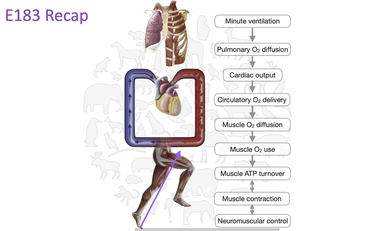
Diagram of a running human figure with the heart and torso highlighted, beside a vertical flowchart listing the integrated steps that determine exercise capacity: minute ventilation → pulmonary O₂ diffusion → cardiac output → circulatory O₂ delivery → muscle O₂ diffusion → muscle O₂ use → muscle ATP turnover → muscle contraction → neuromuscular control.

  • The course examined the physiological systems and principles that determine and limit the ability to perform exercise, from oxygen supply through muscle contraction to neuromuscular control.
  • The focus is largely on humans but placed in a comparative and evolutionary context, which reveals where these systems show adaptability and plasticity versus specialization for particular functions.

Slide 3

Comparative Approaches: The Krogh Principle

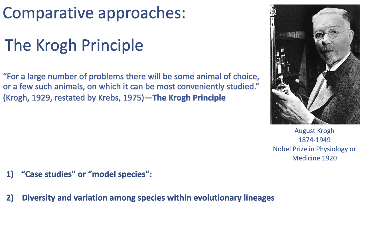
Slide titled "Comparative approaches: The Krogh Principle" with a portrait of August Krogh (1874–1949, Nobel Prize in Physiology or Medicine 1920). A quotation reads: "For a large number of problems there will be some animal of choice, or a few such animals, on which it can be most conveniently studied" (Krogh, 1929, restated by Krebs, 1975). Two approaches are listed: (1) "case studies" or "model species"; (2) diversity and variation among species within evolutionary lineages.

  • The Krogh Principle holds that for many problems there is an ideal animal in which a physiological principle can be most conveniently studied (review Lecture 1).
  • Two comparative strategies recur through the course: case-study or model species (e.g., the cheetah for speed), and broader analysis of diversity and variation within evolutionary lineages.

Slide 4

Diversity of Form Reflects Adaptation and Evolutionary History

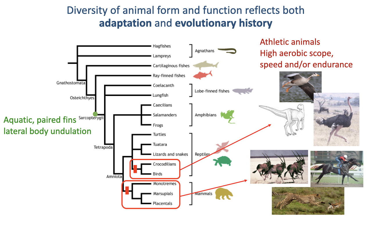
Phylogenetic tree of vertebrates from jawless fishes through tetrapods to mammals and birds, with photos of representative animals. Labels note that the vertebrate origin was aquatic with paired fins and lateral body undulation, and that athletic animals with high aerobic scope, speed, and/or endurance arose among two terrestrial groups — mammals and the archosaur lineage leading to dinosaurs and birds.

  • Animal form and function reflect both adaptation and evolutionary history (review Lecture 1).
  • Vertebrates originated as aquatic animals; high-aerobic, athletic capacity evolved independently in two terrestrial lineages — mammals and the archosaurs (leading to dinosaurs and modern birds) — showing both convergent features and informative differences.

Slide 5

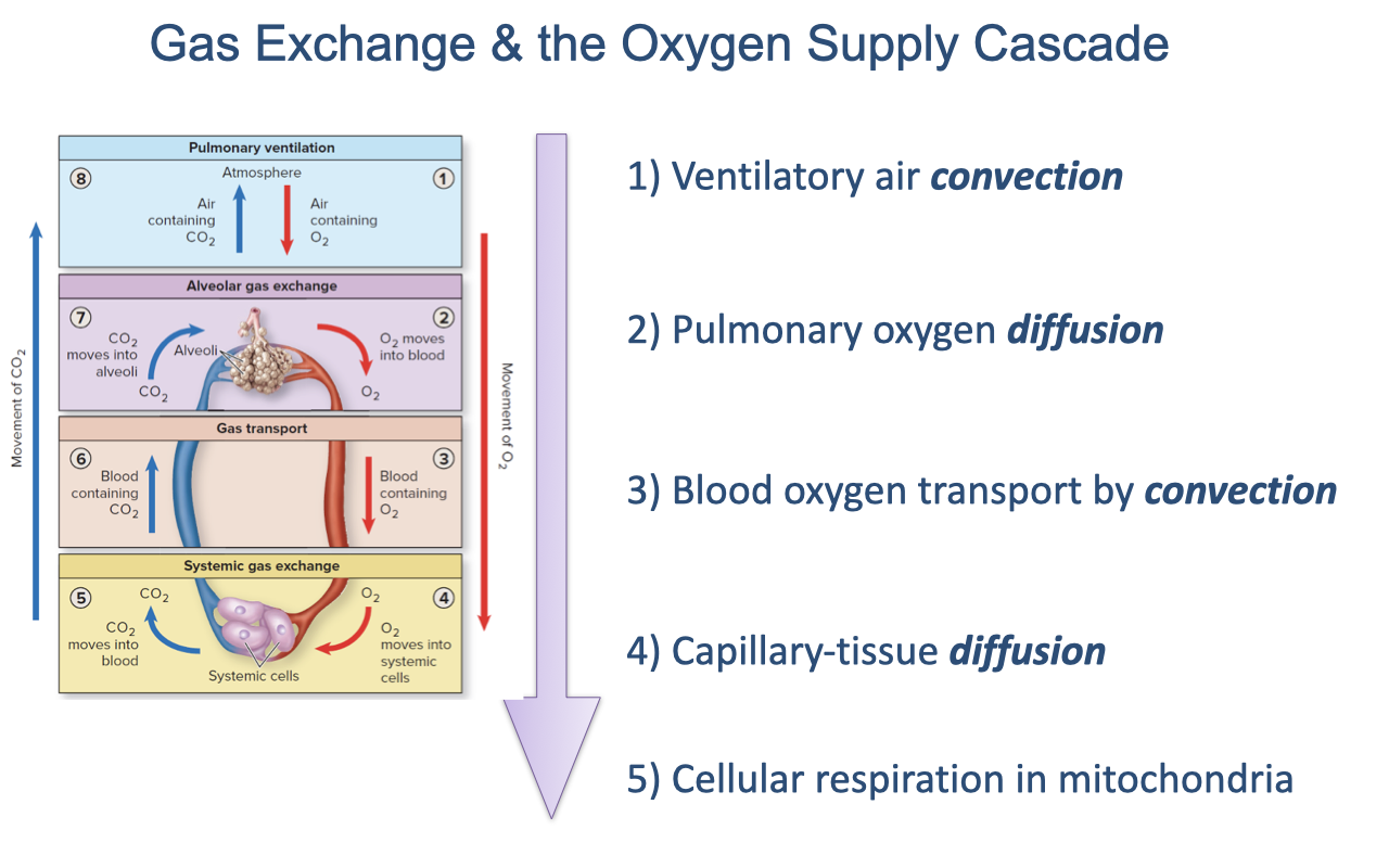
Gas Exchange and the Oxygen Supply Cascade

Diagram of the oxygen supply cascade with four stacked boxes — pulmonary ventilation, alveolar gas exchange, gas transport, and systemic gas exchange — and arrows showing O₂ moving inward and CO₂ moving outward. To the right, the five numbered steps are listed: (1) ventilatory air convection; (2) pulmonary oxygen diffusion; (3) blood oxygen transport by convection; (4) capillary-tissue diffusion; (5) cellular respiration in mitochondria.

  • About four weeks covered the oxygen supply cascade — its sequential steps, governing equations, and limiting factors (review Lectures 1–10).
  • The five steps alternate convection and diffusion: ventilatory air convection, pulmonary diffusion, blood transport by convection, capillary-tissue diffusion, and mitochondrial respiration.
  • Partial pressure of oxygen falls at each step; mitochondrial O2 use is the sink that drives the cascade.

Slide 6

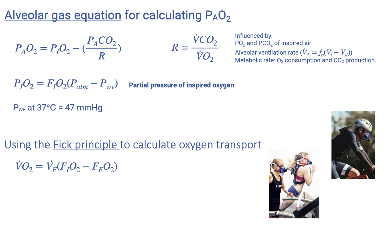
Two Key Equations: Alveolar Gas and the Fick Principle

Slide showing the alveolar gas equation $P_AO_2 = P_IO_2 - (P_ACO_2 / R)$ with the respiratory exchange ratio $R = \dot{V}CO_2 / \dot{V}O_2$, the inspired oxygen term $P_IO_2 = F_IO_2(P_{atm} - P_{wv})$ with water vapor pressure 47 mmHg at 37 °C, and the Fick principle for oxygen transport $\dot{V}O_2 = \dot{V}_E(F_IO_2 - F_EO_2)$. A note lists the factors influencing alveolar oxygen: inspired gas pressures, alveolar ventilation rate, and metabolic rate. Photos show athletes wearing metabolic measurement masks.

  • The alveolar gas equation predicts alveolar oxygen from inspired oxygen, alveolar CO2, and the respiratory exchange ratio $R$ (typically 0.7–1.0); solving it requires the inspired fraction (~21%), atmospheric pressure (altitude-dependent), and water vapor pressure (~47 mmHg) (review Lecture 4).
  • The Fick principle calculates oxygen transport; the fractional-concentration form is preferred for exercise because ventilation and inspired/expired gas fractions can be measured non-invasively with a mask (review Lecture 4).

Slide 7

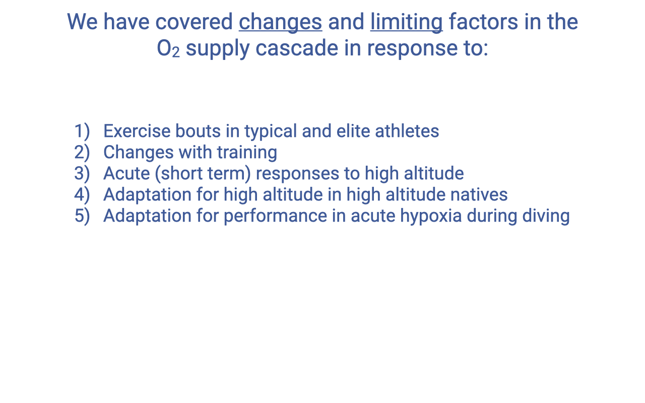
Changes and Limiting Factors in the Oxygen Cascade

Slide titled "We have covered changes and limiting factors in the O₂ supply cascade in response to:" with a numbered list: (1) exercise bouts in typical and elite athletes; (2) changes with training; (3) acute (short term) responses to high altitude; (4) adaptation for high altitude in high altitude natives; (5) adaptation for performance in acute hypoxia during diving.

  • The course examined how each cascade step changes, and what limits it, across five conditions (review Lectures 4–10).
  • These include exercise bouts in typical versus elite athletes, training adaptations (minute ventilation, stroke volume, heart rate), acute high-altitude responses in lowlanders, adaptations in high-altitude natives, and adaptations for acute hypoxia in diving.

Slide 8

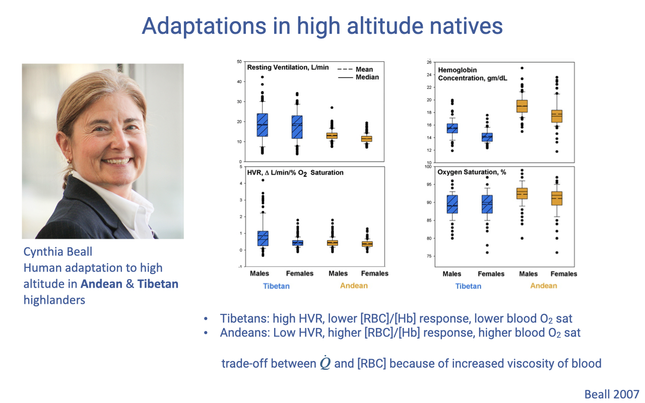
Adaptations in High-Altitude Natives: Tibetan vs. Andean

Slide titled "Adaptations in high altitude natives" with a portrait of Cynthia Beall (human adaptation to high altitude in Andean and Tibetan highlanders) and box-and-whisker plots comparing resting ventilation, hypoxic ventilatory response, hemoglobin concentration, and oxygen saturation between populations. Bullets state: Tibetans have high hypoxic ventilatory response, lower red blood cell count, and lower O₂ saturation; Andeans have low hypoxic ventilatory response, higher red blood cell count, and higher O₂ saturation. A note describes a trade-off between cardiac output and red blood cell count because of increased viscosity of blood. Source: Beall 2007.

  • Different high-altitude human populations evolved different solutions to chronic hypoxia (review Lecture 9).
  • Tibetans show high ventilation and hypoxic ventilatory response but lower red cell count and saturation; Andeans show lower ventilation but higher red cell count and saturation.
  • A functional trade-off prevents combining both: high red cell count raises blood viscosity and cardiac work, and high ventilation demands high cardiac output for ventilation-perfusion matching — so each solution alone aids oxygen delivery and infant survival, but combined they are detrimental.

Slide 9

High-Altitude Adaptations in Bar-Headed Geese

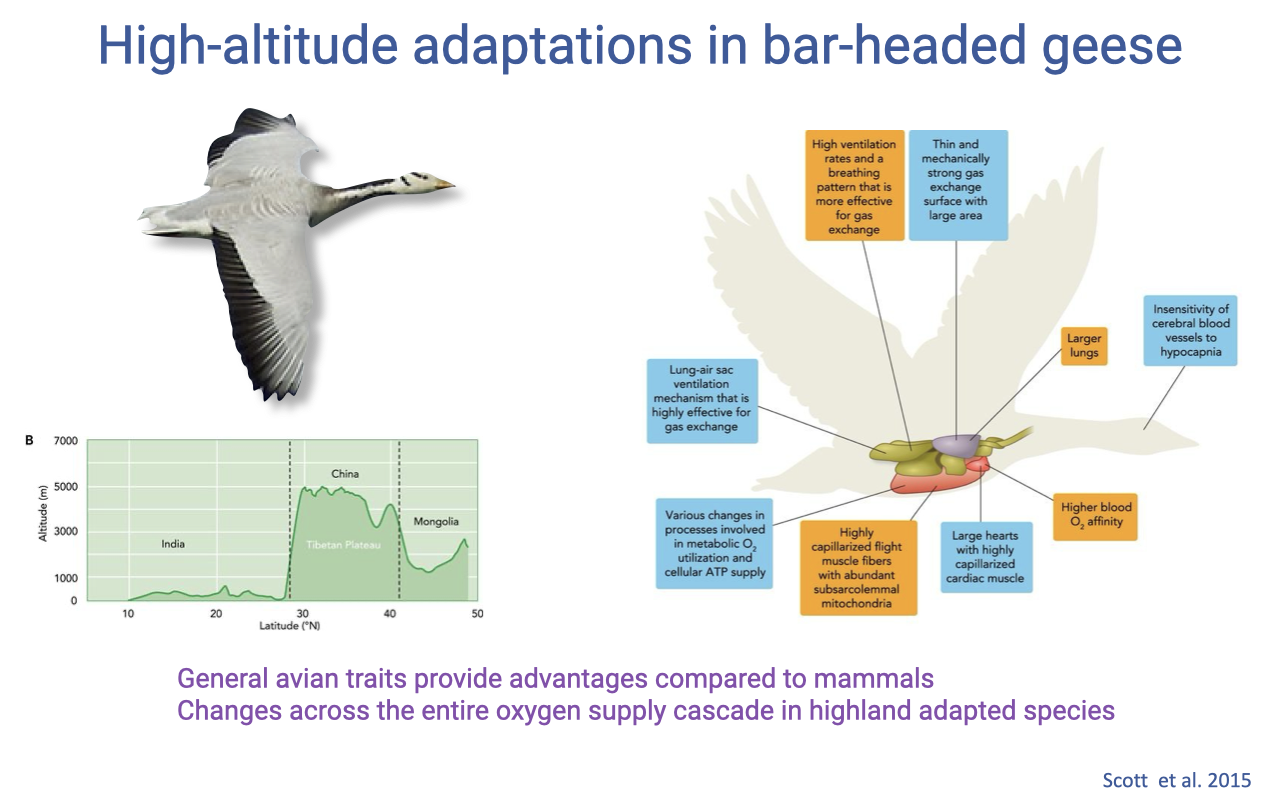
Slide titled "High-altitude adaptations in bar-headed geese" with a photo of a flying goose, a map profile showing the high Tibetan Plateau between India and Mongolia, and a labeled bird diagram listing traits: high ventilation rate and effective breathing pattern, thin gas-exchange surface with large area, larger lungs, insensitivity of cerebral blood vessels to hypocapnia, higher blood O₂ affinity, large hearts with highly capillarized cardiac muscle, highly capillarized flight muscle with abundant subsarcolemmal mitochondria, and a lung–air sac ventilation mechanism. Source: Scott et al. 2015.

  • Birds reach far higher altitudes than mammals, aided by general avian features — air sacs and a rigid lung that lowers the diffusion barrier without needing highly elastic, expandable lung tissue (review Lectures 6 and 9).
  • In highland-adapted species such as the bar-headed goose, advantageous changes occur across the entire oxygen supply cascade, not at one step alone.

Slide 10

Acute Hypoxia: Adaptations for Diving in Mammals

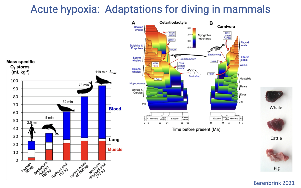
Slide titled "Acute hypoxia: Adaptations for diving in mammals" with a bar chart of mass-specific oxygen stores (mL O₂ per kg) partitioned among blood, lung, and muscle across species from small mammals to elite divers such as seals and whales, showing large increases in blood and muscle stores in divers. Adjacent panels trace the evolution of diving in cetartiodactyls and carnivores over time, with photos of a whale, cattle, and a pig. Source: Berenbrink 2021.

  • Because ventilation is impossible underwater, diving performance depends on oxygen stored in the tissues rather than ongoing supply (review Lecture 10).
  • Divers have high mass-specific O2 stores, chiefly in blood (red blood cells, often released from large spleens during a dive) and in muscle (via myoglobin).
  • A surface-charge change in myoglobin, evolved independently several times, allows tighter myoglobin packing and the characteristically dark-red muscle of deep divers.

Slide 11

Adaptations for Diving in Humans: The Bajau

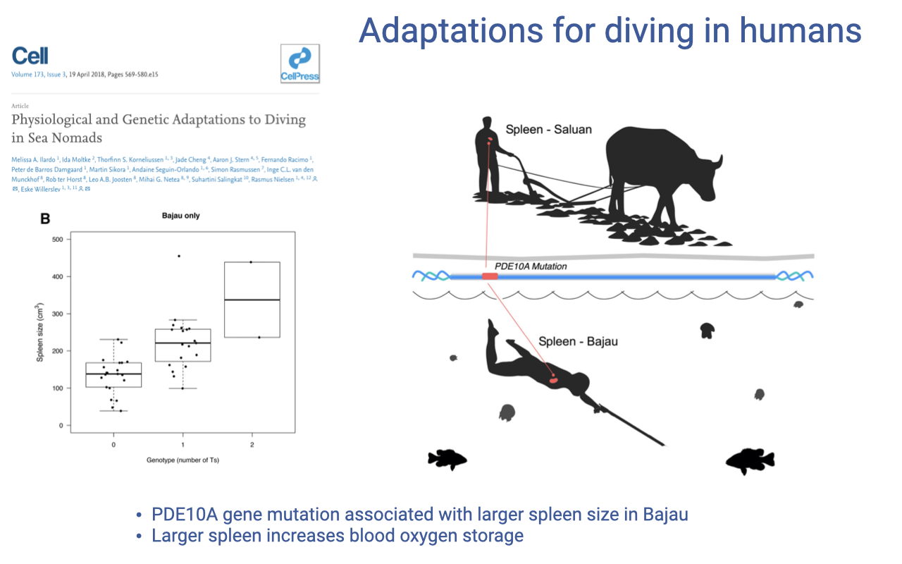
Slide titled "Adaptations for diving in humans" referencing a Cell paper, "Physiological and Genetic Adaptations to Diving in Sea Nomads." A schematic contrasts a non-diving Saluan and a diving Bajau, marking a PDE10A mutation, and a box plot shows spleen size increasing with the number of the associated genotype alleles. Bullets state that the PDE10A gene mutation is associated with larger spleen size in the Bajau, and that a larger spleen increases blood oxygen storage.

  • The Bajau “sea nomads” are persistent breath-hold divers who hold some of the longest human dive records (review Lecture 10).
  • A PDE10A gene variant in this population is associated with larger spleen size, providing extra red-cell oxygen storage that enhances diving performance.

Slide 12

Transition: Muscle Structure and Function

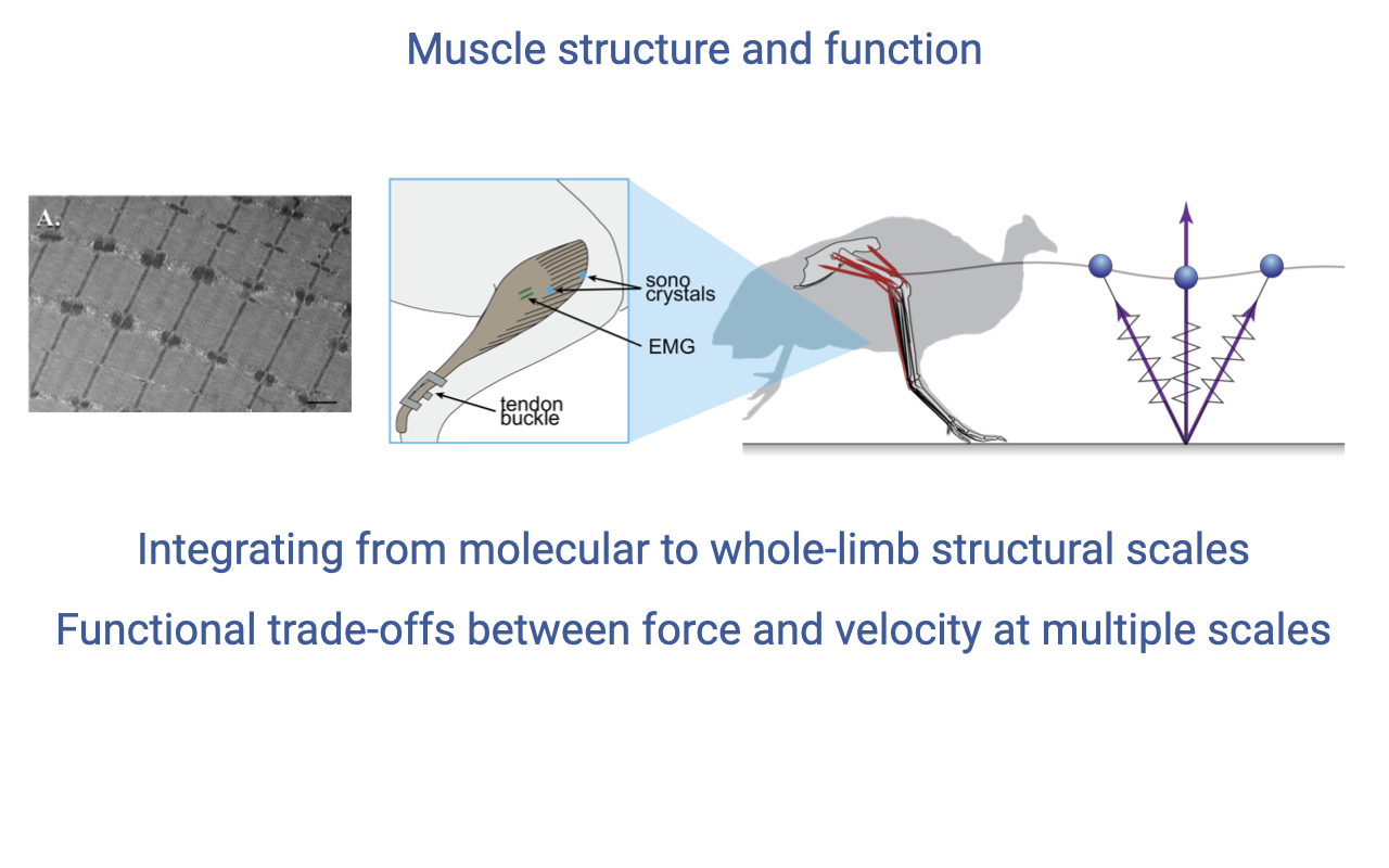
Slide titled "Muscle structure and function" with three images spanning scales: an electron micrograph of sarcomeres, a limb diagram showing sonomicrometry crystals, EMG electrodes, and a tendon buckle, and a running bird with limb force vectors. Text notes the integration from molecular to whole-limb structural scales and functional trade-offs between force and velocity at multiple scales.

  • The second half of the course shifted to muscle — the only motor in the system — progressing from molecular mechanisms up to whole-limb structure (review Lectures 11–18).
  • A unifying theme: force–velocity trade-offs appear at every scale and are additive, so each level contributes to whole-organism performance.

Slide 13

Design Trade-offs in Muscle Cells: The “Zero-Sum Game”

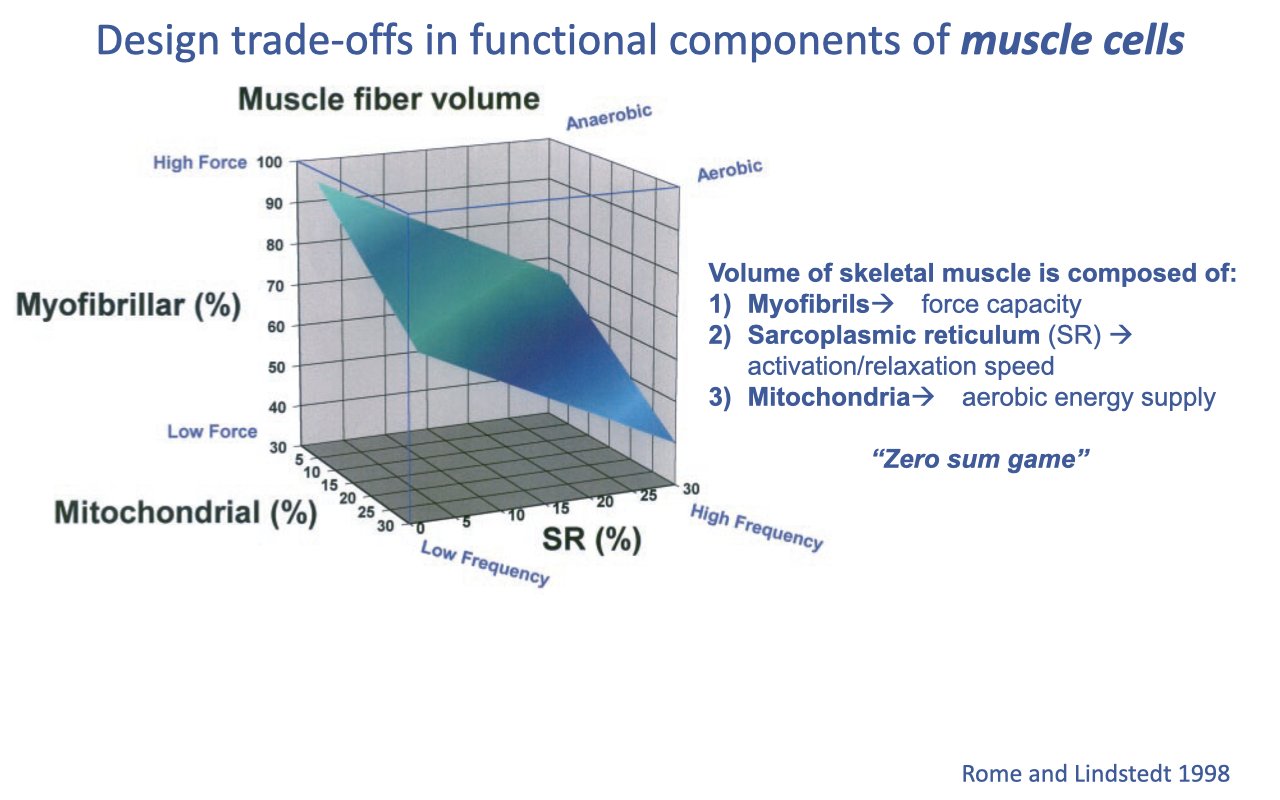
Slide titled "Design trade-offs in functional components of muscle cells" with a 3-D surface plot of muscle fiber volume showing axes for myofibrillar percent, mitochondrial percent, and sarcoplasmic reticulum (SR) percent, with corners labeled high force/low force and aerobic/anaerobic. Text states that skeletal muscle volume is composed of myofibrils (force capacity), sarcoplasmic reticulum (activation/relaxation speed), and mitochondria (aerobic energy supply), described as a "zero-sum game." Source: Rome and Lindstedt 1998.

  • Inside a muscle cell, the volume fractions of myofibrils (force), sarcoplasmic reticulum (activation/relaxation speed), and mitochondria (aerobic capacity) compete — a “zero-sum game” for cell volume (review Lecture 11).
  • This is zero-sum only for volume allocation, not total size — hypertrophy still raises force by adding bulk. The trade-off explains why aerobic muscles, packed with mitochondria, generate lower force, underlying the strength-versus-endurance trade-off.

Slide 14

Intrinsic Contractile Properties of Muscle Tissue

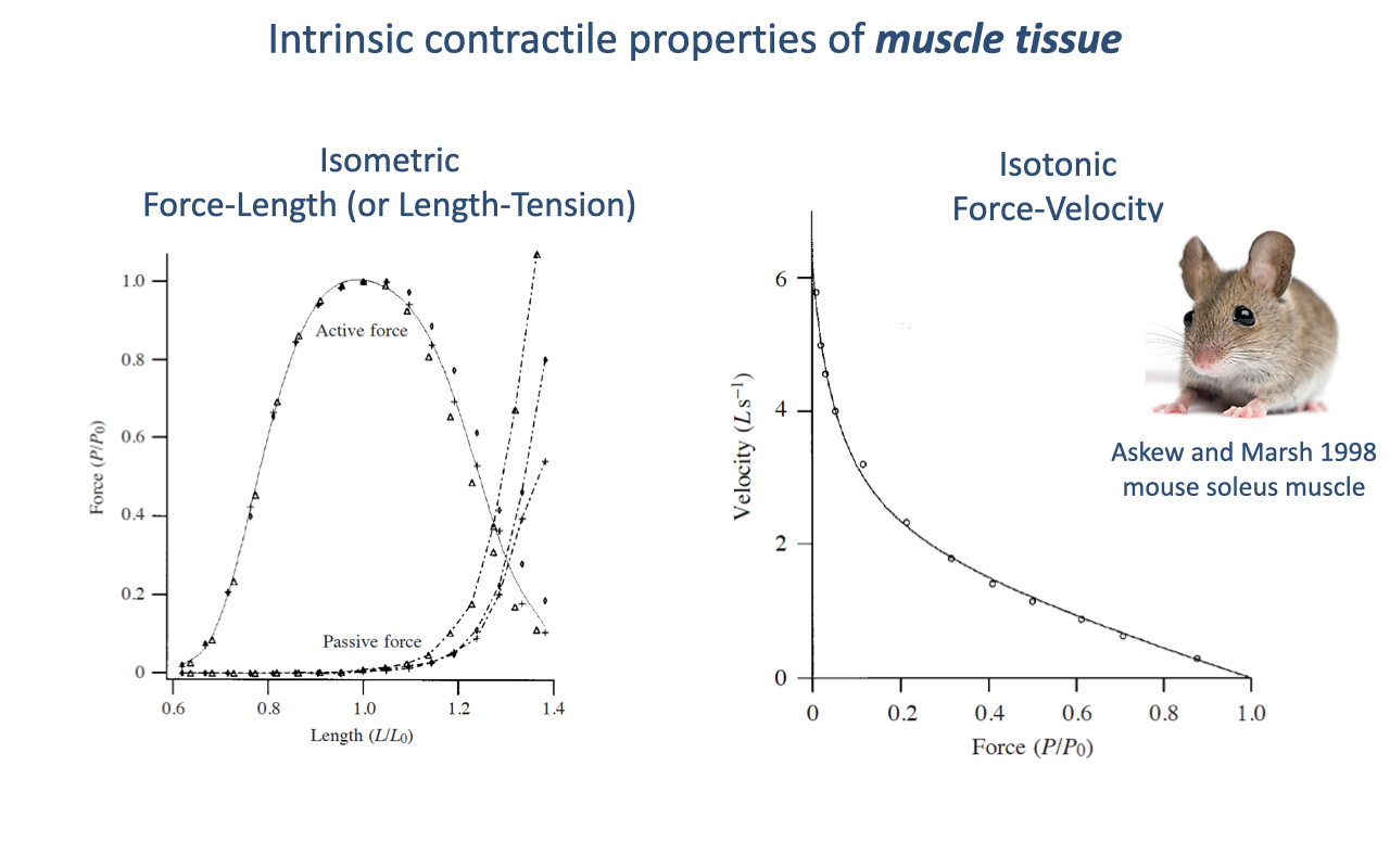
Slide titled "Intrinsic contractile properties of muscle tissue" with two graphs. Left: an isometric force-length (length-tension) curve showing active force peaking near optimal length (L/L₀ ≈ 1.0) and falling off at shorter and longer lengths, plus a rising passive force curve. Right: an isotonic force-velocity curve (mouse soleus, Askew and Marsh 1998) showing velocity declining hyperbolically as force increases.

  • The force–length relationship sets a performance envelope: peak force occurs near optimal length and falls at shorter or longer lengths, so muscles generate force over only a limited excursion (review Lecture 12).
  • The force–velocity relationship shows an inherent force-versus-speed trade-off; because power is force times velocity, peak power occurs at intermediate contraction speeds.

Slide 15

Comparative Maximum Velocity and Body Size

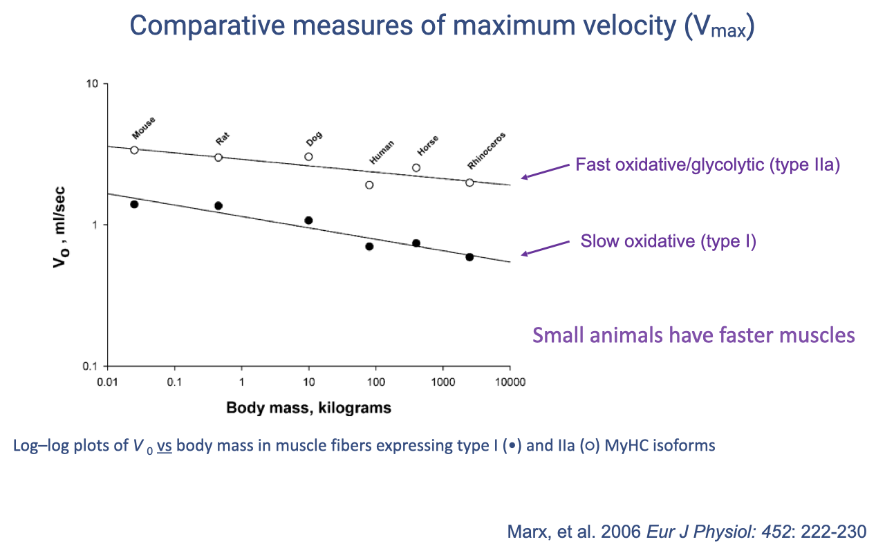
Slide titled "Comparative measures of maximum velocity (Vmax)" with a log–log plot of unloaded shortening velocity (V₀, mL/sec) versus body mass (kilograms) for mouse, rat, dog, human, horse, and rhinoceros. Two parallel declining lines distinguish fast oxidative/glycolytic (type IIa) fibers from slow oxidative (type I) fibers. Text reads "Small animals have faster muscles." Source: Marx et al. 2006.

  • Maximum (unloaded) shortening velocity differs by fiber type — fast versus slow — and also scales with body size (review Lecture 12).
  • Smaller animals have faster muscles; larger animals have slower muscles, partly because larger animals are constrained to trade speed for the force needed to support body weight.

Slide 16

Influence of Anatomy on Muscle-Tendon Function

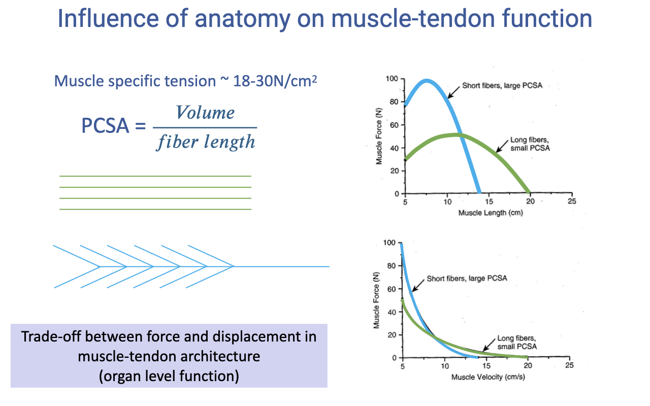
Slide titled "Influence of anatomy on muscle-tendon function" stating muscle specific tension is about 18–30 N/cm² and giving the physiological cross-sectional area as PCSA = Volume / fiber length. Diagrams contrast a parallel-fibered muscle with a pennate muscle. Two graphs compare short-fiber, large-PCSA muscle (high peak force over a narrow length and velocity range) with long-fiber, small-PCSA muscle (lower force over a broader range). Text notes the trade-off between force and displacement in muscle-tendon architecture at the organ level.

  • Specific tension (~18–30 N/cm²) is fairly conserved, so physiological cross-sectional area (PCSA) — volume divided by fiber length — sets a muscle’s force capacity (review Lecture 13).
  • For equal volume, pennate (short-fiber) muscles produce higher force but less displacement, while parallel (long-fiber) muscles produce more displacement and velocity — an organ-level force-versus-displacement trade-off.

Slide 17

Proximo-Distal Distribution of Muscle Mass

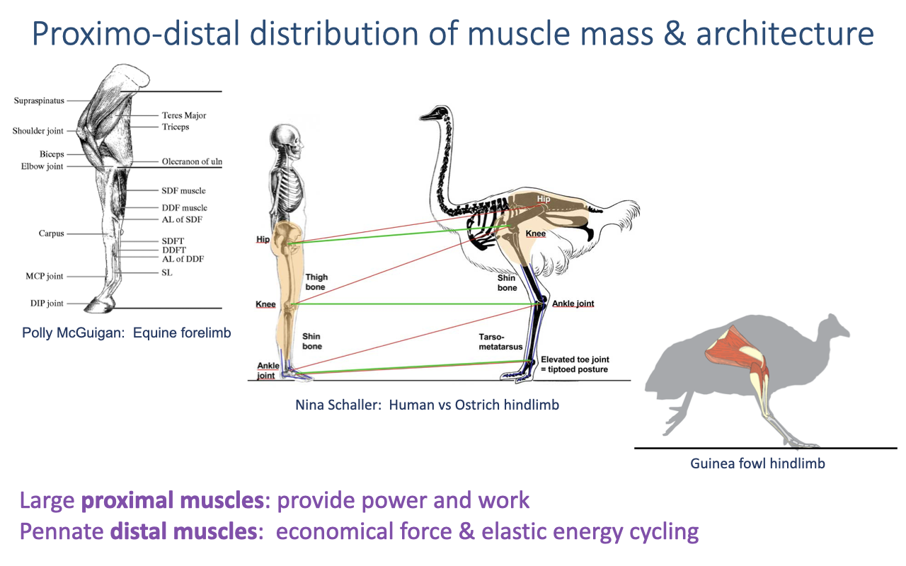
Slide titled "Proximo-distal distribution of muscle mass and architecture" comparing an equine forelimb (Polly McGuigan), a human-versus-ostrich hindlimb (Nina Schaller), and a guinea fowl hindlimb. Bullets read: large proximal muscles provide power and work; pennate distal muscles provide economical force and elastic energy cycling.

  • Limbs distribute muscle architecture by joint position rather than using one generalist design (review Lectures 13–14).
  • Large proximal muscles (hip, knee) have parallel fibers and large volume for high work and power; pennate distal muscles (e.g., calf) give economical force and elastic energy cycling.
  • Keeping distal limbs light reduces limb inertia and the energy cost of swinging the leg.

Slide 18

Integrative Muscle Function: Work Loops

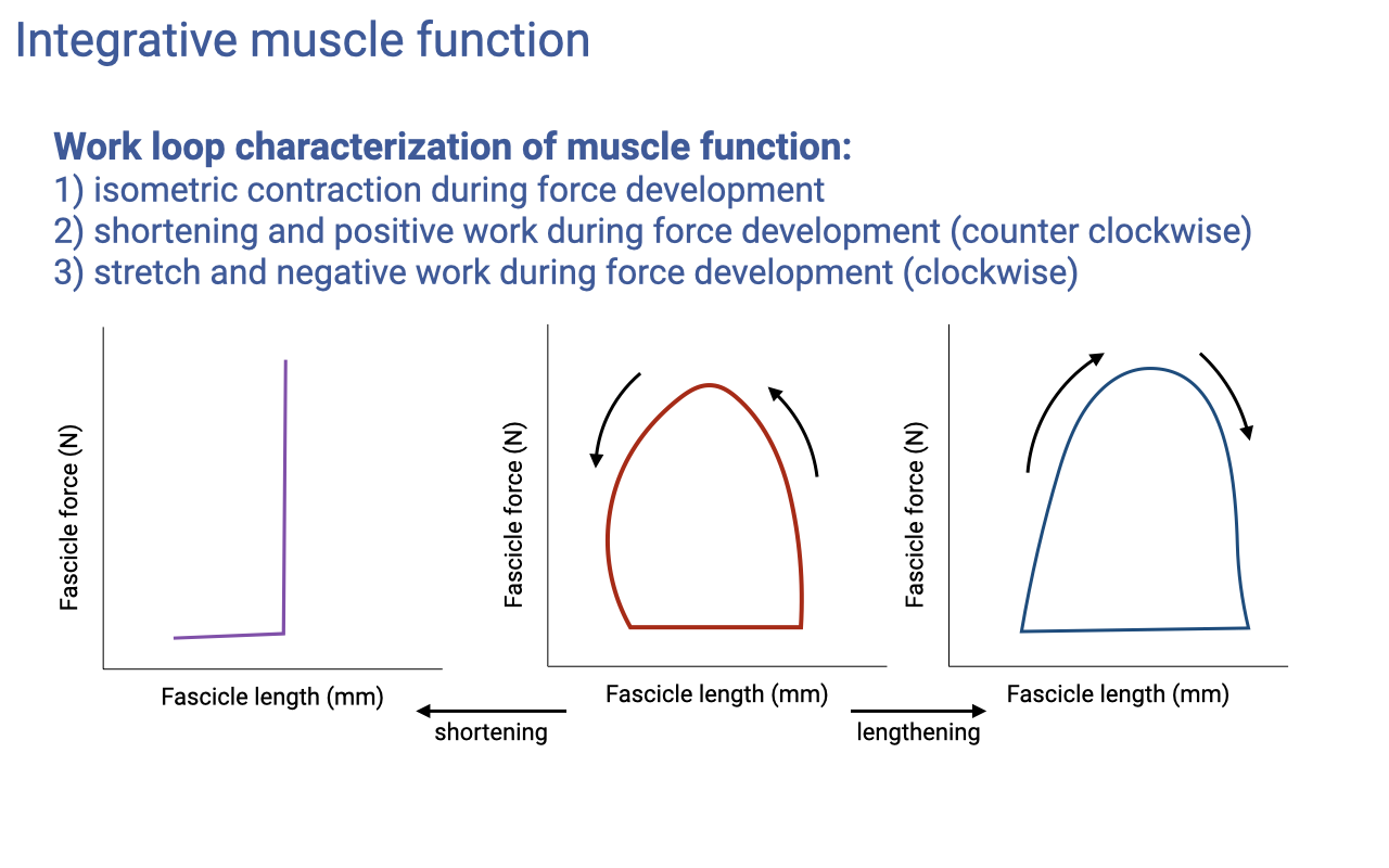
Slide titled "Integrative muscle function" describing work loop characterization with three plots of fascicle force versus fascicle length. Left: a near-vertical line for isometric contraction. Middle: a counter-clockwise loop for shortening with positive work. Right: a clockwise loop for stretch with negative (absorbed) work. Arrows indicate shortening and lengthening directions.

  • Work loops classify muscle action by the shape traced in force–length space (review Lecture 14).
  • Isometric (strut-like, near-vertical) muscles let springy tendons cycle elastic energy; counter-clockwise loops do positive work (motor-like, e.g., bird pectoralis, human hip); clockwise loops absorb energy (brake-like, e.g., landing from a jump).

Slide 19

In Vivo Muscle Function in Humans

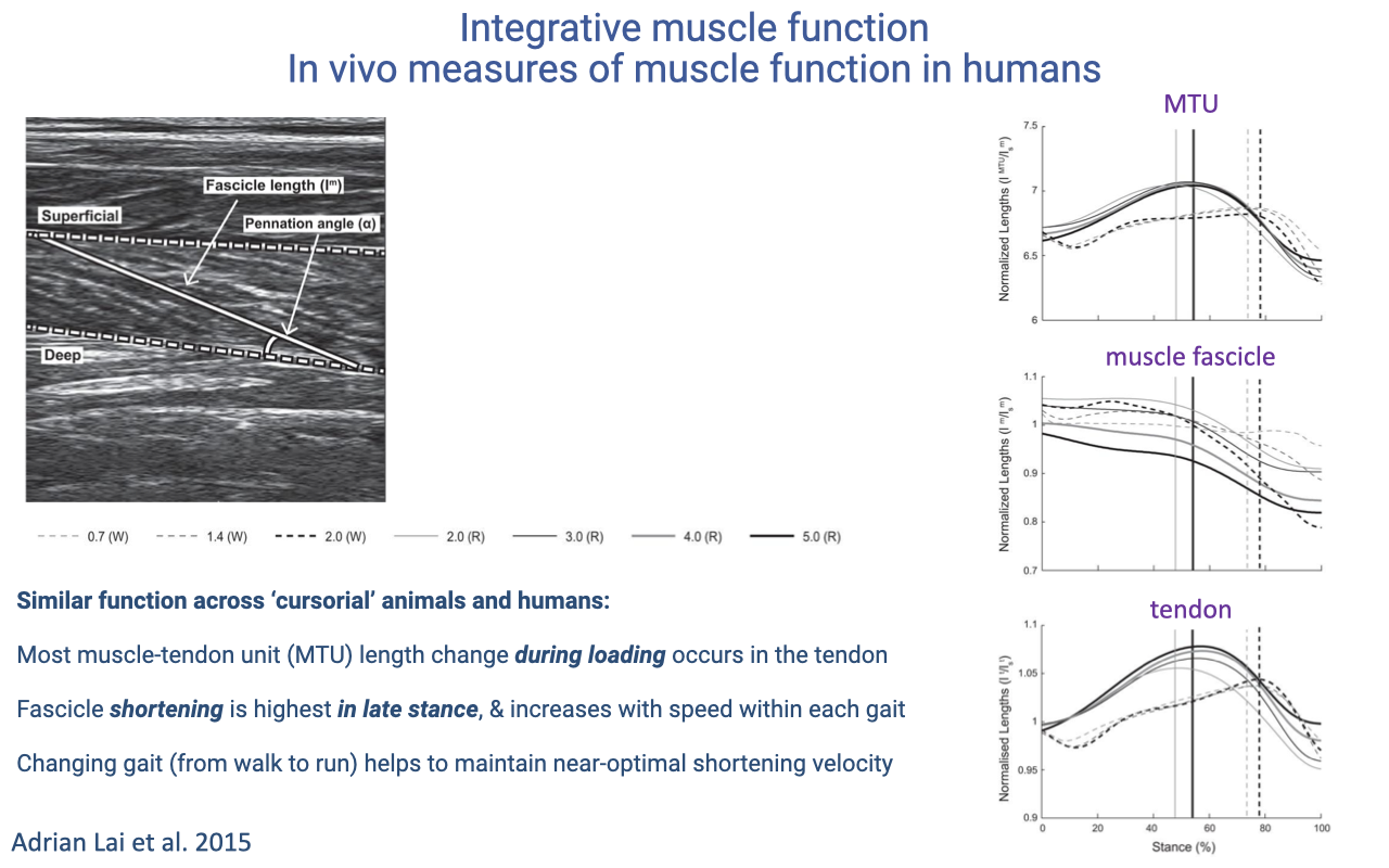
Slide titled "Integrative muscle function: in vivo measures of muscle function in humans" with an ultrasound image of the muscle-tendon unit and three time-series plots of length change for the whole muscle-tendon unit (MTU), the muscle fascicle, and the tendon during stance. Bullets note similar function across cursorial animals and humans: most MTU length change occurs in the tendon during loading; fascicle shortening is highest in late stance and increases with speed within a gait; the gait transition (walk to run) helps maintain near-optimal shortening velocity. Source: Adrian Lai et al. 2015.

  • Ultrasound studies of the human calf reveal that during the first half of stance the tendon stretches while fascicles stay near-isometric; positive fascicle shortening occurs mostly in late stance to re-accelerate the body (review Lecture 14).
  • Fascicle shortening rises with speed within a gait; switching from walking to running keeps fascicle velocity in a more efficient range by shifting load and stretch into the elastic tendons.

Slide 20

Integrated Limb Function: Musculoskeletal Lever Systems

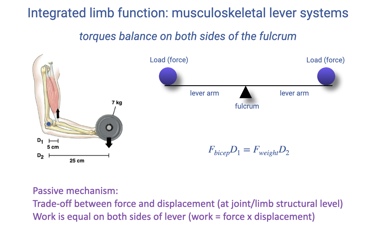
Slide titled "Integrated limb function: musculoskeletal lever systems" stating that torques balance on both sides of the fulcrum. A biceps-and-forearm diagram lifts a 7 kg load with lever arms D₁ = 5 cm and D₂ = 25 cm, and the balance equation is written as $F_{bicep} D_1 = F_{weight} D_2$. Text notes this is a passive mechanism with a force-displacement trade-off, where work is equal on both sides because work equals force times displacement.

  • A lever system balances torques across the fulcrum: muscle force times its moment arm equals load force times its moment arm (review Lecture 14).
  • As a passive mechanism it trades force for displacement but conserves total work — a high-force, low-excursion arrangement versus a low-force, high-excursion one.

Slide 21

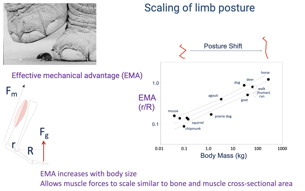
Scaling of Limb Posture

Slide titled "Scaling of limb posture" with a photo of an elephant foot beside a small rodent, a limb diagram defining effective mechanical advantage (EMA) as the ratio r/R of muscle and ground-reaction moment arms, and a log–log plot of EMA versus body mass (mouse and chipmunk through dog and horse) showing EMA rising with size. Text notes a posture shift and that EMA increases with body size, allowing muscle forces to scale similarly to bone and muscle cross-sectional area.

  • Across body size there is a posture shift from crouched (flexed) limbs in small animals to straighter limbs in large animals (review Lecture 14).
  • This raises effective mechanical advantage (EMA) with size, letting muscle force scale in step with bone and muscle cross-sectional area so large animals can support their weight against gravity.

Slide 22

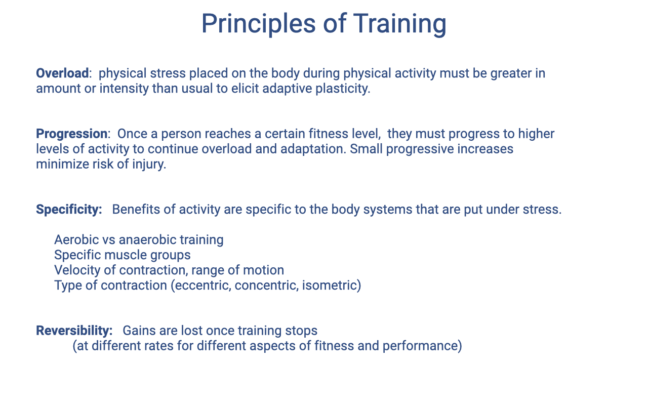
Principles of Training

Slide titled "Principles of Training" defining four principles. Overload: physical stress must exceed the usual amount or intensity to elicit adaptive plasticity. Progression: as fitness improves, activity must increase to continue overload, with small increases to minimize injury risk. Specificity: benefits are specific to the systems stressed — aerobic vs anaerobic, specific muscle groups, velocity and range of motion, and contraction type (eccentric, concentric, isometric). Reversibility: gains are lost once training stops, at different rates for different aspects of fitness.

  • Four training principles govern adaptation (review Lectures 15 and 21): overload (stress beyond the usual), progression (gradually increasing load), specificity (adaptations match the system and movement trained), and reversibility (detraining when training stops).
  • Different forms of activity produce training responses on different timescales, and detraining likewise proceeds at different rates for different aspects of fitness — for example, VO2 and strength are lost at different rates.

Slide 23

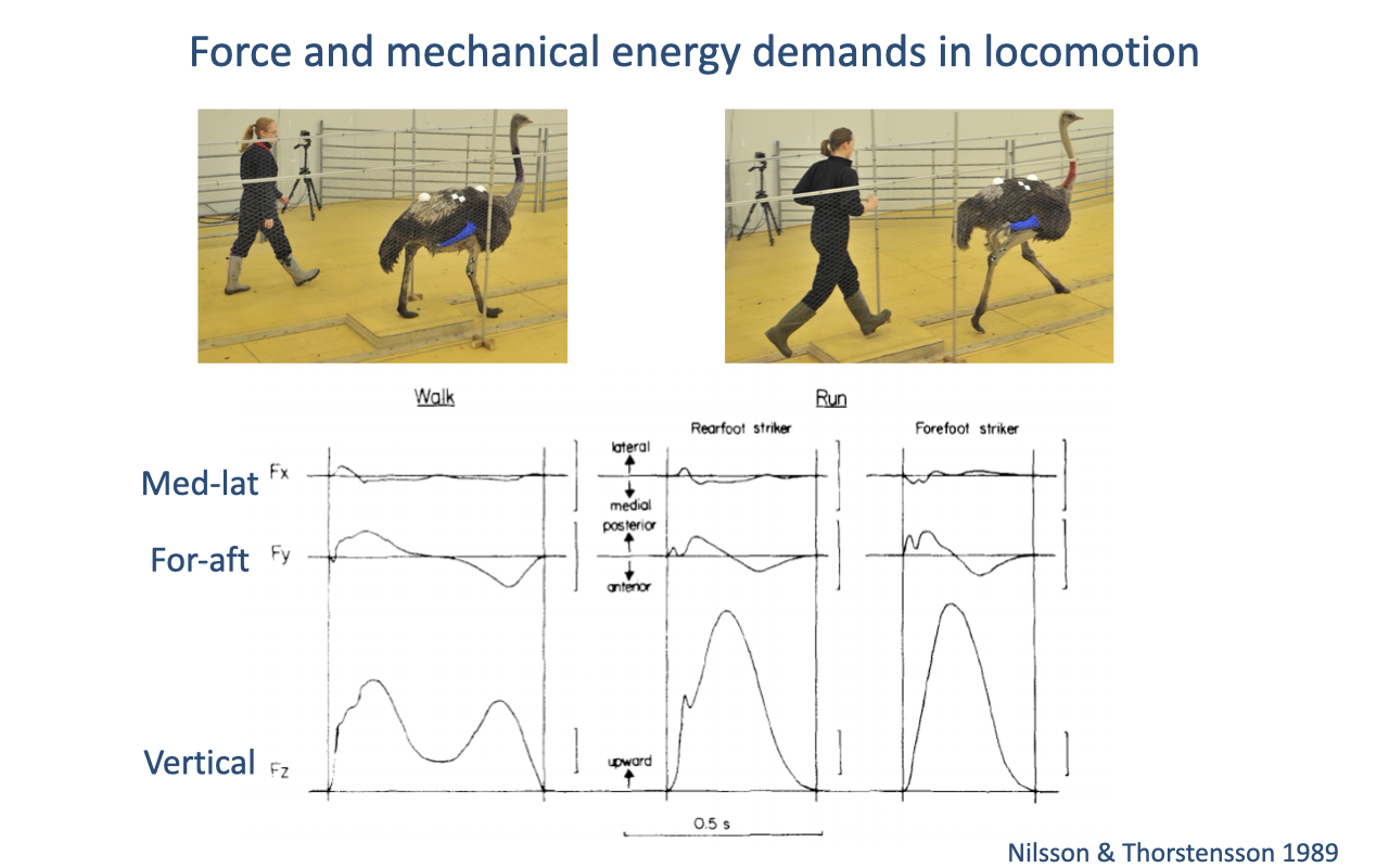
Force and Mechanical Energy Demands in Locomotion

Slide titled "Force and mechanical energy demands in locomotion" with photos of an ostrich walking and running and traces of the three ground reaction force components — mediolateral, fore-aft, and vertical — across a stride for both gaits. Source: Nilsson and Thorstensson 1989.

  • Ground reaction forces have vertical, fore-aft (braking then propulsive), and mediolateral components that vary with gait (review Lectures 16–17).
  • Ground reaction force demands determine the muscle forces required, and therefore the effort and energetic cost of locomotion.

Slide 24

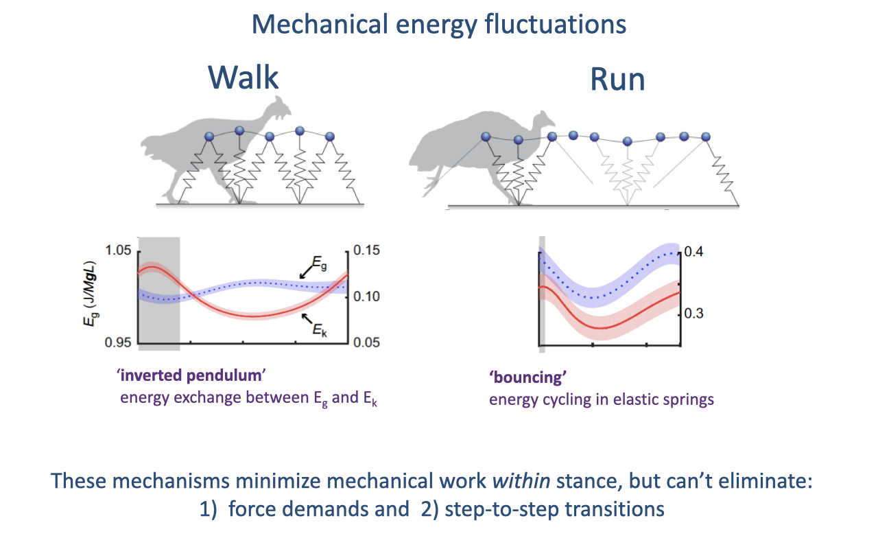
Mechanical Energy Fluctuations: Walking vs. Running

Slide titled "Mechanical energy fluctuations" comparing walk and run with spring-loaded inverted-pendulum diagrams of a bird and plots of gravitational potential energy (E_g) and kinetic energy (E_k) over a stride. In walking the two energies fluctuate out of phase (inverted pendulum exchange); in running they fluctuate in phase (bouncing, elastic energy cycling). Text notes these mechanisms minimize mechanical work within stance but cannot eliminate force demands or step-to-step transition costs.

  • Walking uses inverted-pendulum exchange between gravitational potential and kinetic energy (out of phase); running uses elastic bouncing where the two energies fluctuate in phase (review Lecture 17).
  • Both passive mechanisms reduce the mechanical work of locomotion but cannot eliminate the force demands of supporting body weight or the collisional energy losses of step-to-step transitions.

Slide 25

Energetic Cost of Transport

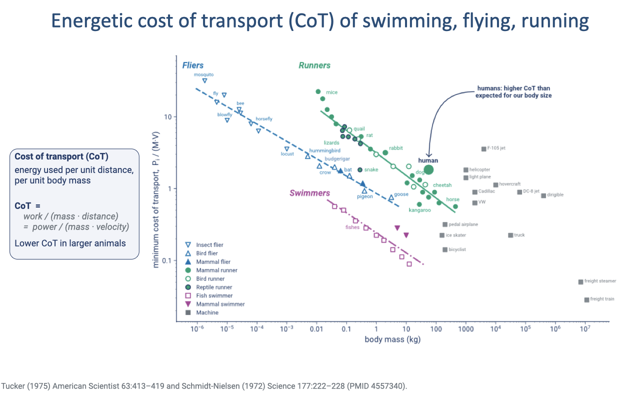
Slide titled "Energetic cost of transport (CoT) of swimming, flying, running" with a log–log plot of minimum cost of transport versus body mass for fliers, runners, and swimmers, plus machines. A box defines cost of transport as energy used per unit distance per unit body mass, CoT = work/(mass × distance) = power/(mass × velocity). An arrow notes humans have higher CoT than expected for their body size. Sources: Tucker 1975; Schmidt-Nielsen 1972.

  • Cost of transport (CoT) is energy used per unit distance per unit body mass; for a given mode it declines with body size — larger animals move more economically per kilogram (review Lecture 18).
  • Running is most costly, flying intermediate, and swimming cheapest, because the force demands differ by mode: runners support body weight against gravity and suffer collisional losses at each foot contact, fliers support weight without collisional losses, and swimmers need not support weight at all.
  • Humans sit somewhat above the expected running line for their size.

Slide 26

Energetics of Running: A Cost-Coefficient View

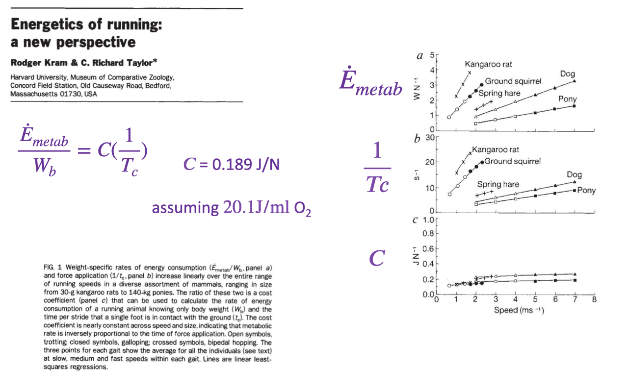
Slide titled "Energetics of running: a new perspective" (Kram and Taylor) giving metabolic rate per body weight as $\dot{E}_{metab} / W_b = C(1/T_c)$, with cost coefficient C ≈ 0.189 J/N assuming 20.1 J per mL O₂. Graphs plot metabolic rate and its inverse against the inverse of foot-ground contact time (1/T_c) for a kangaroo rat, ground squirrel, spring hare, dog, and pony, showing a consistent linear relationship.

  • Kram and Taylor showed that running metabolic rate scales with the rate of force generation — the inverse of foot-ground contact time, $1/T_c$ (review Lecture 18).
  • A nearly constant cost coefficient (~0.189 J/N) links the energy cost to how quickly the limbs must be cycled to apply support force.

Slide 27

Why Larger Animals Have Lower Cost of Transport

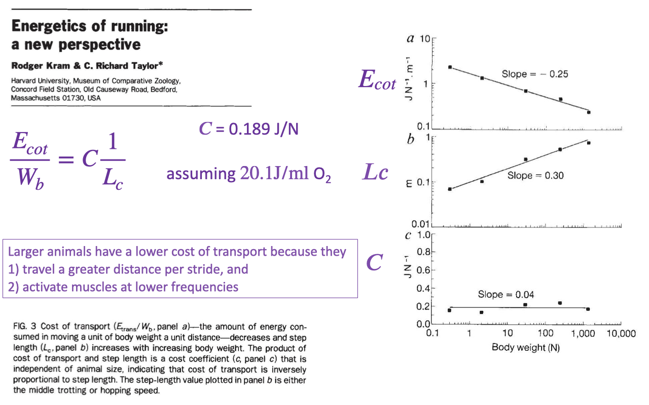
Slide titled "Energetics of running: a new perspective" with graphs of the cost coefficient C and length term Lc versus body weight, showing slopes near 0.25–0.30 across body sizes from small mammals to large ones. Text explains that larger animals have lower cost of transport because they travel a greater distance per stride and activate muscles at lower contraction frequencies.

  • Larger animals have lower cost of transport because they cover more distance per stride and turn their muscles on and off at lower frequencies, giving longer ground-contact times and lower force-generation costs (review Lecture 18).
  • The cost coefficient stays roughly constant across body size, and the same scaling has been replicated within humans of differing stature.

Slide 28

Gait Selection and the Energetics of Locomotion

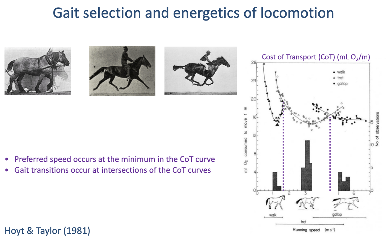
Slide titled "Gait selection and energetics of locomotion" with Eadweard Muybridge photo sequences of a horse walking, trotting, and galloping, and a plot of cost of transport versus running speed showing separate U-shaped curves for walk, trot, and gallop. Bullets state that preferred speed occurs at the minimum of each CoT curve and that gait transitions occur at the intersections of the curves. Source: Hoyt and Taylor 1981.

  • Within a gait, cost of transport follows a U-shaped curve when animals are forced off their preferred speed — moving faster or slower than preferred both raise the cost (review Lecture 18).
  • Preferred speeds occur at each curve’s minimum, and gait transitions occur where adjacent curves intersect, which requires projecting the curves to locate the crossing points.

Slide 29

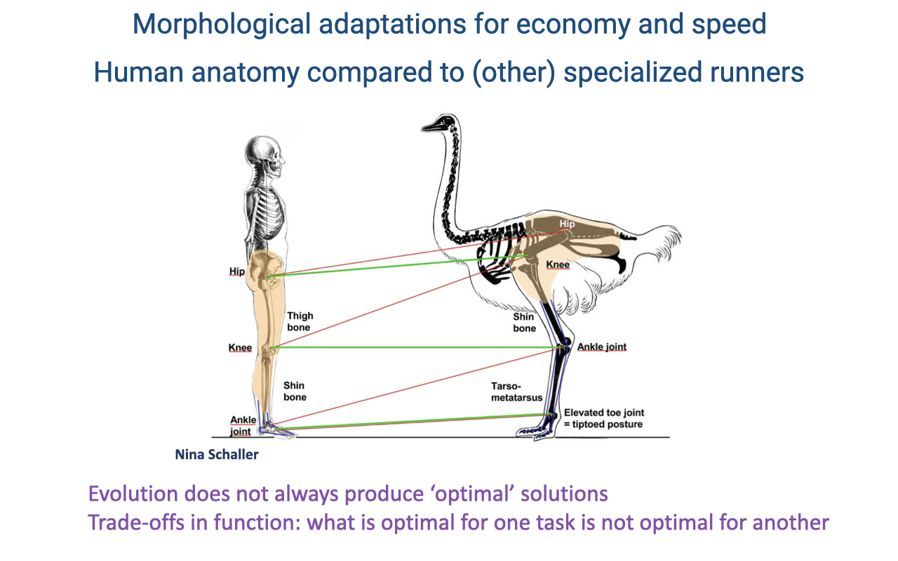
Morphological Adaptations for Economy and Speed

Slide titled "Morphological adaptations for economy and speed: human anatomy compared to (other) specialized runners" comparing a human skeleton with an ostrich skeleton, with colored lines linking corresponding hip, knee, and ankle joints and noting the ostrich's elevated, tip-toed toe joint. Text reads: evolution does not always produce optimal solutions; trade-offs in function mean what is optimal for one task is not optimal for another. Source: Nina Schaller.

  • Athletic demands differ: migrating long distances favors economy, while escaping predators favors speed — some features serve both, but not all (review Lecture 18).
  • Whether humans count as specialized runners is debated. Humans have long legs (suggesting athletic specialization) but heavy, massive legs compared with specialized runners such as the ostrich.
  • Evolution does not always produce optimal solutions — it tinkers with inherited form, so human function must be read against our primate ancestry, and trade-offs mean what is optimal for running need not be optimal for walking or non-locomotor tasks.

Slide 30

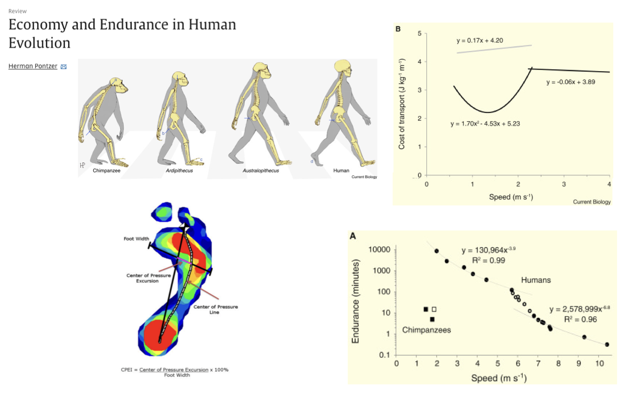
Economy and Endurance in Human Evolution

Slide titled "Economy and Endurance in Human Evolution" (Herman Pontzer) showing a series of increasingly upright hominins from chimpanzee through Ardipithecus and Australopithecus to modern human. A graph plots cost of transport versus speed with a U-shaped curve for human walking, a foot center-of-pressure heatmap, and a log–log plot of endurance time versus speed comparing humans and chimpanzees. Source: Current Biology.

  • Placed against great-ape ancestry, humans have exceptionally economical walking — a much lower cost of transport than chimpanzees, with a clear U-shaped optimum (review Lecture 18).
  • Humans also show exceptional endurance in both walking and running, along with physiological specializations such as heat dissipation that support sustained activity — consistent with selection for economical, enduring movement.

Slide 31

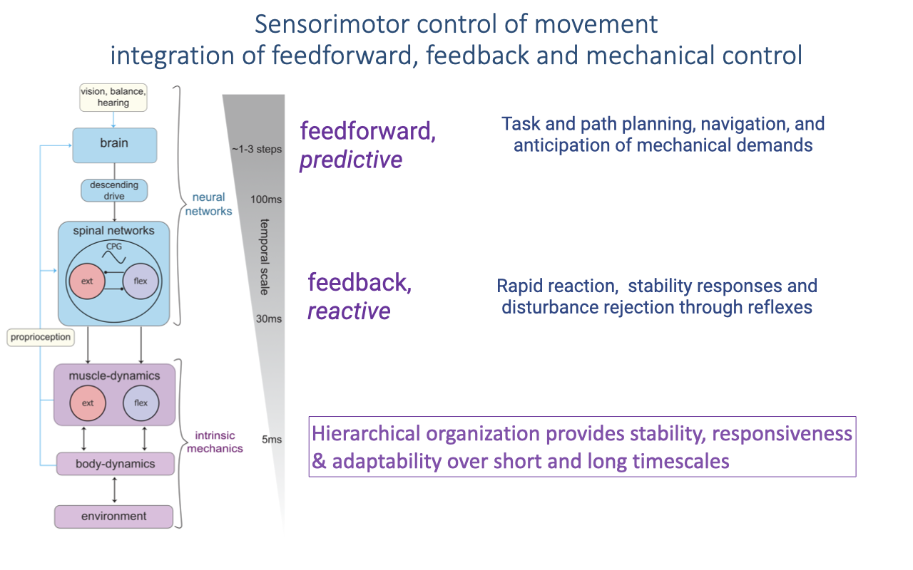
Sensorimotor Control of Movement

Slide titled "Sensorimotor control of movement: integration of feedforward, feedback and mechanical control" with a hierarchical diagram linking environment, body dynamics, muscle dynamics, spinal networks (with a central pattern generator and extensor/flexor units), the brain, and sensory inputs (vision, balance, hearing, proprioception). A temporal scale runs from ~5 ms intrinsic mechanics through 30–100 ms reflexes to 1–3 step planning. Feedforward (predictive) control handles task and path planning; feedback (reactive) control handles rapid stability and disturbance rejection. Text notes the hierarchy provides stability, responsiveness, and adaptability across timescales.

  • Locomotor control integrates feedforward (predictive) planning, feedback (reactive) reflexes, and intrinsic mechanical responses, organized hierarchically across timescales from ~5 ms to several steps (review Lecture 20).
  • This layered organization provides stability, responsiveness, and adaptability simultaneously.

Slide 32

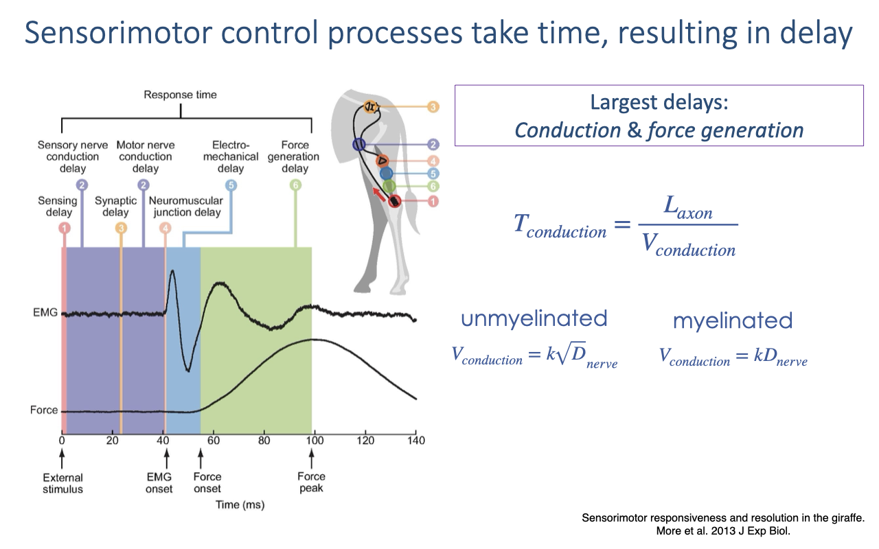
Sensorimotor Control Takes Time

Slide titled "Sensorimotor control processes take time, resulting in delay" with a timeline of response components — sensory and motor nerve conduction delay, synaptic delay, neuromuscular junction delay, electromechanical delay, and force-generation delay — aligned to EMG and force traces over about 140 ms. Equations give conduction time as $T_{conduction} = L_{axon} / V_{conduction}$, with unmyelinated conduction velocity scaling as the square root of nerve diameter and myelinated velocity scaling linearly with diameter. Text notes the largest delays come from conduction and force generation. Source: More et al. 2013, J Exp Biol.

  • Each control step adds delay — sensory and motor conduction, synaptic and neuromuscular-junction transmission, and electromechanical plus force-generation delay (review Lecture 20).
  • Conduction time depends on axon length and velocity (faster in larger and myelinated axons); the largest contributions are nerve conduction and force generation.

Slide 33

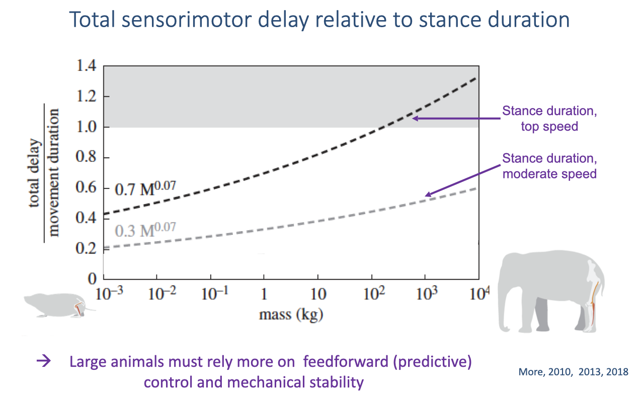
Total Sensorimotor Delay Relative to Stance Duration

Slide titled "Total sensorimotor delay relative to stance duration" with a plot of the ratio of total delay to movement duration versus body mass (from a small rodent to an elephant). Two dashed curves, scaling as roughly mass to the 0.07 power, represent top-speed and moderate-speed stance durations; delay approaches or exceeds stance duration in the largest animals. Text reads: large animals must rely more on feedforward (predictive) control and mechanical stability. Source: More 2010, 2013, 2018.

  • Sensorimotor delay grows relative to stance duration as body size increases, so feedback corrections arrive too late within a step for the largest animals (review Lecture 20).
  • Large animals must therefore rely more on feedforward (predictive) control and intrinsic mechanical stability.
  • Humans fall on the larger side of this scaling, so at fast running speeds reflexes are too slow and movement must be planned predictively — a demand that may have contributed to the evolution of larger brains.

Slide 34

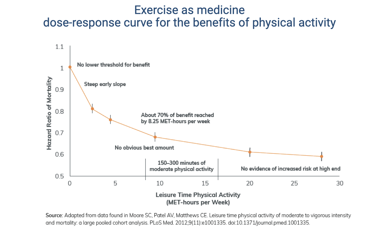
Exercise as Medicine: The Dose-Response Curve

Slide titled "Exercise as medicine: dose-response curve for the benefits of physical activity" with a plot of hazard ratio of mortality versus leisure-time physical activity (MET-hours per week). The curve falls steeply at first and flattens, annotated: no lower threshold for benefit, steep early slope, about 70% of benefit reached by 8.25 MET-hours per week, no obvious best amount, 150–300 minutes of moderate activity, and no evidence of increased risk at the high end. Source: adapted from Moore et al., PLoS Med 2012.

  • Physical activity reduces mortality risk along a dose-response curve with no lower threshold and a steep early benefit — roughly 70% of the maximum benefit is reached near 8.25 MET-hours per week (review Lecture 21).
  • Benefits continue with more activity, with no clear optimal dose and no evidence of harm at the high end, assuming energetic needs are met and adequate rest avoids injury.
  • Across the population, higher activity is associated not only with lower mortality but also lower chronic-disease and cancer risk, better cancer survivability, and improved cognitive function and mood regulation.

Slide 35

Closing slide reading "Questions?" in large blue text on a white background.

  • The recap closes by inviting questions and encouraging students to revisit the lectures noted above to synthesize the course’s major themes — comparative and evolutionary context, the oxygen supply cascade, muscle structure and function across scales, the mechanics and energetics of locomotion, sensorimotor control, and exercise as medicine.